ABSTRACT
SMITH, KARL WILLIAM. The Prior Trap. (Under the direction of Stephen Margolis).
Basic economic theory suggests that the decision to go to college should be based only on the
expected costs and benefits of college. The income of the family the student comes from
should have no effect. Yet, it does. The two common explanations for this discrepancy,
inadequate primary school funding and liquidity constraints are at odds with the facts. I offer
a third explanation, economically disadvantaged students attend college at lower rates
because they have biased information. This analysis connects to the existing literature in at
least three ways. It provides a rational basis for the neighborhood effect., extends work on
human capital development indicating that educational paths are set at or before age 16 and
helps provide an explanation for the both the increase in the return to education and the
The Prior Trap
by
Karl William Smith
A dissertation submitted to the Graduate Faculty of North Carolina State University
in partial fulfillment of the requirements for the Degree of
Doctor of Philosophy
Economics
Raleigh, North Carolina
2007
APPROVED BY:
__________________ __________________
Stephen Margolis Charles Knoeber
Chair of Advisory Committee
__________________ __________________
ii
DEDICATION
This work is dedicated to my future wife Larisa Yasinovskaya, who has been my partner, my
confidant, my conscience and my best friend throughout this entire project. It was through
her that I learned I could fake my way through a life unexamined. It was because of her that I
set my targets outside of the expertise of my department. It was because of her that I had the
courage to pursue this project without regard to its marketability. She has stuck by my side
through the good and perhaps mostly bad times that it took to get this far.
iii
BIOGRAPHY
It is often said that good writers know what to write, great writers know what to steal. And,
so I steal from the best.
Three passions, simple but overwhelmingly strong, have governed my life: the longing for
love, the search for knowledge, and unbearable pity for the suffering of mankind. These
passions, like great winds, have blown me hither and thither, in a wayward course, over a
great ocean of anguish, reaching to the very verge of despair.
I have sought love, first, because it brings ecstasy - ecstasy so great that I would often have
sacrificed all the rest of life for a few hours of this joy. I have sought it, next, because it
relieves loneliness--that terrible loneliness in which one shivering consciousness looks over
the rim of the world into the cold unfathomable lifeless abyss. I have sought it finally,
because in the union of love I have seen, in a mystic miniature, the prefiguring vision of the
heaven that saints and poets have imagined. This is what I sought, and though it might seem
too good for human life, this is what--at last--I have found.
With equal passion I have sought knowledge. I have wished to understand the hearts of men.
I have wished to know why the stars shine. And I have tried to apprehend the Pythagorean
power by which number holds sway above the flux. A little of this, but not much, I have
iv Love and knowledge, so far as they were possible, led upward toward the heavens. But
always pity brought me back to earth. Echoes of cries of pain reverberate in my heart.
Children in famine, victims tortured by oppressors, helpless old people a burden to their sons,
and the whole world of loneliness, poverty, and pain make a mockery of what human life
should be. I long to alleviate this evil, but I cannot, and I too suffer.
This has been my life. I have found it worth living, and would gladly live it again if the
v
ACKNOWLEGEMENTS
I’d like to thank my mother, my sister, my father who is no longer with us, Ed Whitfield, and
Leon Watson for supporting my annoying insatiable questioning from a young age. I thank
Mike McElroy, John Lapp, John Seater, Kerry Smith and Patti Clayton for that same support
at a slightly older age. I thank my committee for tolerating my work habits. A special thanks
goes to Steve Margolis for always inviting me back to his office, no matter what I had done
since my last visit. This was truly much more than anyone could reasonably ask for. I thank
Pat Inman for increasing the probability that someone might actually be able to understand
vi
TABLE OF CONTENTS
LIST OF FIGURES ... vii
INTRODUCTION ... 1
THE INFORMATION PROBLEM THAT STUDENTS FACE ... 4
BACKGROUND TRENDS ... 12
COMPETING EXPLANATIONS FOR LOW COLLEGE GOING RATES ... 20
ANALYTICAL MODEL... 29
How Communities Become Educated ... 39
How do Some Communities Remain Uneducated? ... 46
Why Would Graduating Agents Not Return to the Community? ... 52
The Truly Disadvantaged ... 53
Several Puzzles Solved ... 56
Lower Levels and a Slower Response ... 60
NUMERICAL SIMULATION ... 61
Model Structure ... 63
Results ... 69
CONCLUSIONS... 81
vii
LIST OF FIGURES
Figure 1. Change in Earnings and Attendance ... 12
Figure 2. College Participation ... 14
Figure 3. College Participation by Race ... 16
Figure 4. Two Year College Attendance ... 17
Figure 5. Perceptions Locus ... 37
Figure 6 . Intergenerational Dynamics ... 43
Figure 7. Dynamics with Alpha ... 48
Figure 8. Shallow vs. Step Perceptions ... 51
Figure 9. Alpha at Zero ... 55
Figure 10. Multiple Equilibria ... 58
Figure 11. Simulated Curves ... 59
Figure 12. Simulated Graduation Rates ... 70
Figure 13. Simulated Study Rates ... 71
Figure 14. Simulate Wage Premium ... 72
Figure 15. Simulated Income Ratio ... 73
Figure 16. Simulated Graduation Fraction ... 74
Figure 17. Simulation with Vietnam Effect ... 76
Figure 18. Wages with Vietnam ... 77
1
INTRODUCTION
The lower a student’s income the less likely the student is to attend college. Basic
economic theory suggests that the decision to go to college should be based on a
comparison of the gains that a student expects to receive from going to college with the
costs associated with preparation and attendance. The income of the family the student
comes from should have no effect. Yet, it does.
There are two common explanations for the observed relationship between family income
and college attendance, but both are at odds with the facts. The first is that students
economically disadvantaged families do not have the money and cannot borrow the
money to pay for a college education. The evidence suggests, however, that family
income leading up to and during college is a much weaker predictor of college attendance
than family income during primary school. The relationship between family income and
future college attendance is established early in a student’s life and so it is unlikely that
liquidity constraints are the involved.
The second explanation is that students from less affluent communities attend less
effective primary schools. The logic is that school funding is determined in part by local
tax revenue and thus students in economically disadvantaged communities will go to
2 have a strong effect on student outcomes. Poorly funded schools in wealthy communities
tend to do better than well funded schools in poor communities.
I offer a third explanation. Economically disadvantaged students go to college at lower
levels because they have different expectations than students raised in more affluent
communities. The community matters not because it determines school funding but
because it determines student expectations. Formally, I argue that economically
disadvantaged students attend college at lower rates because they have biased
information. A key ingredient in college success is preparation. Students will only spend
time and effort preparing for college if they believe that they have reasonable chance of
succeeding. Students who grow up in communities where most adults have not
completed or even attended college rationally conclude that their chances of completing
college are low as well. Therefore, they invest little in college preparation. Because
students have not prepared for college they do not get into college or perhaps more
commonly they don’t even bother applying.
My analysis extends findings in the existing literature in at least three ways. First, it
provides a rational basis for the neighborhood effect. Students “prefer” to act like their
peers and role models because peers and role models provide valuable information about
the optimal way to behave. In short, in a world fraught with uncertainty, group
3 Second, this analysis extends work on human capital development which suggests that
educational paths are set at or before age 16. Heckman and Carnerio find a
crystallization effect during the early teenage years. Keane and Wolpin show that
endowments at age 16 are highly determinate in a young men’s career path.
Third, this paper helps provide an explanation for the both the increase in the return to
education and the slowdown in college graduation growth among young men in the
United States. Card and Lemiuex who show that the increase in the return to education
could be explained two factors, a linear trend in the demand for educated workers and an
exogenous slowdown in the growth rate of the supply of college graduates. The model I
build endogenizes that supply side slowdown.
The rest of the paper proceeds as follows. Chapter 2 provides a non-technical overview of
the student’s information problem. Chapter 3 discusses some background trends in
college going. Chapter 4 looks at some competing explanations for those trends and the
empirical problems with those explanations. Chapter 5 provides a formal model of the
students problem and develops tools for comparative statics of community level behavior.
Chapter 6 outlines and provides the results of a numerical simulation of US white male
college going rates since 1950 based on the analytics of the model developed in Chapter
4
THE INFORMATION PROBLEM THAT STUDENTS FACE
High school students must make numerous choices that could have long lasting
consequences on their earning potential. I focus, however, on one choice: whether or not
to devote time and energy preparing for college.
There are essentially three elements that go into making this choice.
1. The cost of studying
2. The benefits of successfully completing college
3. The probability that the student will finish college if he or she studies
Students who devote more time to studying may complete more years of college, on
average, than those who study less and students who complete some college earn more on
average than students who complete none. To make the analysis as simple as possible,
however, I will present the argument in terms of binary choices and consequences. Either,
the student prepares for college or does not. Either, the student finishes college or does
not. While this reduces the complexity considerably the fundamental issue remains the
same: a student must choose how much time and energy to devote to college preparation
today, in the hopes that he or she will receive some gains in the future.
Rational students will choose to prepare for college if the expected benefits outweigh the
5 studying students could choose to either work, spend time with their friends and family or
engage in other pursuits of their own choosing. Students who choose to devote time to
studying cannot also be working and so must give up whatever wages they would have
earned. Since all students 16 years of age or older have the opportunity to work at the
minimum wage a student must at least give up 5.45 per hour in order to study. However,
some students may value other activities at more than 5.45 an hour. If so those students
are sacrificing even more.
The expected benefits of studying are determined in two steps. The first step is to
calculate the benefits a student can expect if he successfully graduates college. The
second step is to factor in the probability that the student will graduate from college if he
or she prepares. The expected benefit after graduation multiplied times the probability
that of graduation.
In the first, step the student has to add up the value of the extra earnings that a college
graduate receives but subtract out the costs of tuition, books, and lost income during
college. In the second step the student has to form an estimate of the probability of
graduate. It is the student’s difficulties in the second step which form the heart of this
paper. Even, if the benefits from completing college are high the expected benefit can be
6 For example, a student who knows that he or she will receive at net benefit of $250,000
by graduating college but believes that there is a 10% chance of graduating if he or she
studies faces an expected benefit of $25,000. If it costs more than $25,000 in lost part
time work earnings then it will not be worth it to study. While both the benefit and the
probability of graduating may be difficult to calculate, I argue that the student is likely to
be much more uncertain about his chances of graduating than the rewards if he graduates.
A student’s chances of graduating college depend at least in part on his scholastic ability.
How scholastic ability is determined is outside the scope of this paper. It could be
partially genetic or entirely environmental. However, I do assume that by age 16 a
student possesses either scholastic advantages or disadvantages which will affect his
probability of successfully completing college. Students with greater scholastic ability
will have a greater chance of graduating college, but the exact relationship between
scholastic ability and the probability of graduation may be complex and unknown.
I suggest that a priori students do not know the exact relationship between ability and the
probability of graduation. They must back out this relationship by observing the world
around them. The accuracy of the student’s information can affect the choices he makes.
In particular, I argue that residential segregation based on income systematically biases
the information a student has and lead him to make decisions he would not have made if
7 Imagine, once again that a student knows he will earn an extra $250,000 if he or she
graduates from college. To prepare for college he must give up two years of part-time
work or roughly $12,500. If the student believes that his chances of graduating college
are 5% then his expected benefits will be at least (.05)*($250,000) = $12,500. In other
words, a student who believes he has a 5% chance of graduating college if he prepares
will find that the expected benefits are exactly equal to the cost. A student who believes
that he has greater than a 5% chance will find that the expected benefits of preparing for
college outweigh the costs. Conversely, a student who believes that he has less than a 5%
chance of graduating college will find that the benefits are less than the cost. In this way,
the student’s estimate of his chances of completing college become crucial in determining
whether or not he prepares.
A student’s community provides information that will help him determine the probability
that he will graduate from college if he prepares. He knows that his scholastic ability is a
factor. However, he does know the exact relationship between scholastic ability and
probability of success. The student, however, can observe the adults in his community.
He knows whether or not they have graduated from college and he can likely deduce how
their scholastic ability compares to his own. Using this information he can get an idea of
how likely he is to graduate.
As long as the adults in the community are a random sample of the population as a whole
8 right but it will produce a better estimate of the relationship than the proceeding
generation. After a few generations have passed the community will accurately interpret
the relationship between scholastic ability and probability of graduation.
A problem is created, however, if the community is not a random draw from the
population. If the community is created in such a way that college graduates have a
disproportionate chance of either being included or excluded from the community then
the information available to students will be biased. Students will systematically draw the
wrong conclusions. In particular, if college graduates are unlikely to return to a
community then students will underestimate their probability of graduating college. This
will lead to under investments in college preparation and lower graduation rates. In fact,
it is possible for the cycle to feed on itself until a community has no college graduates at
all, and no students or only the students with the very highest aptitudes will prepare for
college.
Since college graduates earn more on average than non-college graduates residential
segregation on the basis of income will bias the distribution of graduates. Economically
disadvantages communities will tend to have fewer college graduates and exhibit the
effects described above. In fact, the greater the gap in earnings between college graduates
and non-graduates the stronger the residential segregation will be and the more biased the
information available to economically disadvantaged students will be. This can produce
9 Student’s would be able to mitigate this effect if other sources of information available to
them beside relative comparisons to others in their community. Absolute measures of
scholastic ability, however, may be hard to come by. Grades are in part a relative measure
of performance. Standardized test scores are available but such tests often measure
accumulated knowledge rather that raw scholastic ability. Students may take the
scholastic aptitude test, however, the relationship between the SAT and college
graduation is debated even among experts.
Perhaps, more to the point accessing and analyzing this information may prove
challenging to a high school student. Parents and teachers can offer advice about how to
analyze this information and which sources to trust, however, talk is literally cheap and it
is difficult to know which sources of information to trust.
It is a teacher’s job to help a student prepare for higher education and thus a student
might expect a teacher to at least give lip service to the advantages of preparation even
when the expected benefits are low. Parents might encourage a student to prepare for
college in an effort to raise the family’s status, to fulfill a dream the parents have or
simply because parents may place a low value on the sacrifices the student must make.
Perhaps most importantly, a student may discount what a parent says because he can
10 telling you that you should make a significant investment in education yet you observe
that this person and this person’s peers have not made that investment it would be
reasonable to question the credibility of that information.
Moreover, many parents from economically distressed communities may not pressure
their children to prepare for college because the parents themselves have low estimates of
the return to education. If the only person encouraging you to prepare is the person who
is paid to prepare you then there are strong reasons to consider that individual’s
information dubious at best. Who is the student to believe, his teacher or his lying eyes.
Unusually persuasive teachers may be able to overcome this trust gap and alter student
expectations. I will return to this point later. Note, however, that this implies that it is a
teacher’s ability to motivate economically disadvantaged students, not instruct them that
makes the difference.
The proposed link between residential segregation based on income and college
preparation can cause some counter-intuitive results in the labor market. For example, if
the gap between the income of college graduates and non-college graduates rises then
there is a greater benefit to completing college. We would expect that this would lead
more students to prepare for college. If, however, this rising gap leads to increased
segregation between college and non-college graduates the number of students preparing
11 Card and Lemieux show that the rapid increase in the earnings gap between college and
non-college workers beginning in the 1980s could be explained by steady growth in the
demand for college educated workers since World War II but declining growth in supply
since the mid 1970s. Increases in residential segregation based on income could serve as
12
BACKGROUND TRENDS
Since 1975 the gap between the wages of college educated workers and non-college
educated workers has grown substantially. However, the number of men who graduate
from college has changed very little. The number of female college graduates has been
growing; however, it is difficult to determine how much of that is due to social rather
than economic forces. Economically disadvantaged and minority men seem have
particularly muted response to the increase in the earnings gap.
Between 1974 and 2000 the earnings ratio between college and non-college educated
American men grew from 1.5 to 2.0, an increase of 33%.
-20.00% -10.00% 0.00% 10.00% 20.00% 30.00% 40.00% 1 9 7 6 1 9 7 7 1 9 7 8 1 9 7 9 1 9 8 0 1 9 8 1 1 9 8 2 1 9 8 3 1 9 8 4 1 9 8 5 1 9 8 6 1 9 8 7 1 9 8 8 1 9 8 9 1 9 9 0 1 9 9 1 1 9 9 2 1 9 9 3 1 9 9 4 1 9 9 5 1 9 9 6 1 9 9 7 1 9 9 8 1 9 9 9 2 0 0 0
Percent Change Relative to 1976 Levels
Earnings Ratio Completion Rate
13 The leading explanation for the increase in the earnings ratio is an increased demand for
skilled workers driven by computer related technological change. For this paper, however,
the more interesting question is why the supply response has been so small.
One might imagine that there was a marginal American man in 1976 for whom the
increased earnings from a college education just failed to overwhelm the costs of tuition
and four years of lost pay and work experience. In the 1990s that same man should have
chosen to enter college but it seems he did not. The completion rate by the end of the
century was nearly identical to 1976 levels.
As Card and Lemieux point out, changes in earnings and enrollment are actually
negatively correlated over much of the period and the effect is even more dramatic when
earnings are restricted to workers under 30. Young workers without a degree saw their
real wages fall slightly while young college educated workers experienced larger wage
increases than their older counter parts.
Card and Lemieux suggest that the slow growth of male college completion since the
1960s rather than computer related technological change is the driving force behind the
increase in earnings inequality. While this is a strong possibility the fact I want to focus
on here is that male college completion, was at a minimum, slow to respond to earnings
14 Of particular interest is that among poorer students college attendance is lower and
seemingly slower to respond to changes in the earnings ratio. The chart below is used
often by James Heckman and is taken from Heckman and Carnerio.
Figure 2 College Participation
The returns to college began to increase in the early 1980s and students from upper
income families responded almost immediately. Students from the third quartile did not
respond until the mid-80s and students from the lowest quartile did not respond until the
15 Racial groups show a similar pattern of levels and response timing. Blacks and Hispanics
have both a lower level of college participation and are slower to respond to increases in
the wage premium. The following chart, also taken from Heckman and Carnerio,
illustrates that black and Hispanic college enrollment did not respond to the increase in
the earnings premium until the late 80s and early 90s respectively.
Both charts, however, are likely to overstate the response of schooling to changes in the
earnings ratio. The CPS enrollment data combines two and four year college enrollment
and makes no adjustment for how long it takes students to finish college.
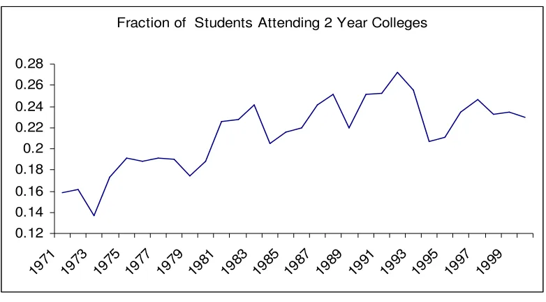
During the early 90s when minority and poor white college enrollment was growing the
fastest, the percentage of students in rolled in two year colleges was at its height. A
portion of the enrollment response is thus likely do to an increase in two year rather than
four year college enrollments. In addition, Bound, Lovenheim and Turner report that for
students in the 1972 National Longitudinal Survey, 51.5% of those who would go on to
earn a baccalaureate degree from a public institution did so by their fourth year out of
high school. In the 1988 National Education Longitudinal Survey that percentage had
16 Therefore, some of the increase in enrollment during the early 90s represents a greater
fraction of two year college students and an increasing number of four year college
students who took longer than four years to graduate.
17 Fraction of Students Attending 2 Year Colleges
0.12 0.14 0.16 0.18 0.2 0.22 0.24 0.26 0.28
1971 1973 1975 1977 1979 1981 1983 1985 1987 1989 1991 1993 1995 1997 1999
Figure 4 Two Year College Attendance
Poor students are more likely to live in the same communities as other poor students and
minorities are more likely to live in the same communities as other minorities. The trends
in college attendance, however, could simply be a result of income and race effects rather
than community induced priors.
Mayer 2000, however, estimated the effect of state level income variance between census
tracts and with-in census tracts on educational outcomes.1 Geographic neighborhoods are not quite the same as communities. Communities exist within social space and have
temporal lags with respect to geography. Individuals may interact frequently with friends
or relatives who live across town and moving to a different geographic neighborhood
does not necessarily produce immediate changes in the social community he or she
1
18 interacts with. There is, nonetheless, a strong correlation between geographic
neighborhoods and social communities. To the extent that an increase in earnings
variance manifests itself as an increase in the variance of earnings between
neighborhoods, communities’ expectations should diverge. Conversely increases in the
variance of earnings inside of neighborhoods should cause less, if any, divergence in
community expectations.
Mayer’s findings support this hypothesis. In her most complete specification, which
includes family income and race, a one standard deviation increase in between tract
income variance yields an estimated increase of .730 years of schooling for students in
the upper half of the income distribution and a decrease of .499 years of schooling for
students in the lower half of the income distribution for a total divergence on 1.229 years
in schooling. On the other hand a one standard deviation increase in within tract variance
results in an estimated increase of .418 years schooling for students in the upper half of
the distribution and no response for students in the lower half of the distribution. Thus,
increases in socioeconomic stratification between neighborhoods seem to encourage
schooling among wealthier students and discourage schooling among poorer students.
There is no way to tell if the distribution of college graduates and the returns to education
are what induce the differences in income variance in Mayer’s study. Nonetheless, the
19 response pattern of income and racial groups to changes in the earnings ratio and this
20
COMPETING EXPLANATIONS FOR LOW COLLEGE GOING RATES
There are two common explanations for low college going rates among economically
disadvantaged students. The first is that students from less affluent communities are not
well prepared for college because of poorly funded primary and secondary schools. The
second is that students simply lack the resources to pay for a college education
Inadequate funding for primary schooling is the most common explanation for the lower
college going rates in economically distressed communities. If those students go to
elementary and middle schools that are lacking resources then they may be unprepared
for high school and therefore correctly estimate that their chances of getting into and
succeeding in college are low.
Hanushek (JEL, 1986) surveys the literature and provides meta-analysis on K12
performance. Of particular interest is the fact that per pupil expenditures on current
services expanded in real terms by 135% between 1960 and 1983. However, measures of
pupil performance declined over that period.
Some of this effect may be due to rising costs. Increasing productivity in the
non-education sectors tends to drive up labor costs in non-education even when the level of service
remains constant. The level of service, however, was not constant over the period.
21 Nonetheless scores on Iowa’s Tests of Educational Development peaked in the late 60s
and declined precipitously into the 1980s. Nationally, the fraction of graduating seniors
going on to college rose from 32.8% in 1960 to 46.1% in 1970 but has remained roughly
constant since. The time series data seem to suggest that resources-per-pupil is not the
dominant factor in determining educational performance.
Hanushek examines 147 studies of school performance based on instructional inputs.
Sixty-five of those studies included per pupil expenditures. In only sixteen where
expenditures significant and in three of those the effect was negative. In only 13 (20%),
did expenditure have a significant positive effect.
To confound matters it is possible that in these few incidences the effect runs the other
way. Suppose that students in less affluent communities do worse because they have
worse expectations. The studies do not include an independent measure of income.
Therefore, to the extent that economically disadvantaged communities have lower
funding the expectations effect could be attributed to school funding.
An empirical regularity mentioned in Hanushek and supported with extensive panel data
in Rivkin, Hanushek and Kain (Econometrica, 2005), is that while per pupil expenditure
22 quality have large effects. This is consistent with the general notion that expectations are
important.
Though not explicitly modeled here, it is conceivable that certain teachers are able to gain
the trust of their students. Information that these teachers provide information will then
be incorporated in a student’s expectations. Teachers who are able to convince students
that effort will be rewarded with a high probability will raise academic performance.
Thus a teacher’s ability to gain the trust of students may serve as the source for
unobserved differences in ability.
The second explanation depends on the concept of liquidity constraints. Liquidity
constraints imply that students are not able to borrow enough money to finance a college
education. If young students could borrow all of the money that they needed then they
could repay the loans with their increased earnings and still be better off. The evidence
for liquidity constraints, however, is weak.
James. J. Heckman argues that cognitive skills become crystallized around the age 14. In
particular, Heckman and Carnerio (2000), presents evidence that family income during
the final years of high school have no effect on college going rates. Instead, family
income during the primary school years seems to be a determining factor. If students
were liquidity constrained then one would expect that losses in income leading up to high
23 not seem to be the case. Either lower family income during primary school sets into
motion some a chain of events that prevents college going or it serves as a proxy for
some deeper effect.
One of the most impressive analyses of college going choices comes from Keane and
Wolpin. The estimate a dynamic programming model of career choices based on data
from the National Longitudinal Survey of Youth (NLSY). There model follows the
choice of young men to go to school, work in white-collar occupation, work in
blue-collar occupations, serve in the military or stay out of the labor force. Their model
accounts for skill and knowledge accumulation and allows for differing preferences
between the young men.
Keane and Wolpin find that 90 percent of the variance in career decision is determined by
and young man’s type laid down by age 16. That is, something happens to young men by
age 16 which will largely guide their career paths for the rest of their lives. There are
four possible types. Type one individuals tend to be the most educated averaging roughly
16 years of education and work almost exclusively in white collar occupations. Type two
and three individuals work mostly in blue collar occupations though type threes spend
some time in the military. Roughly half of type two and three individuals finish high
school and a small fraction goes on to post-secondary education. Type four individuals
24 home. These types are not determined by the researchers but are chosen by the computer
after analyzing patterns in the data.
Most interestingly, types are heavily correlated with parental education and income. The
computer simulation determines types by analyzing patterns in the young men’s behavior.
However, when the researchers compare those types parental education and income they
find that highly educated and affluent parents are much more likely to have type one
children. Lower income and less educated parents were much more likely to have type
three children. The parent of type two individuals had similar education profiles as type
the parents of type three individuals but tended to be slightly higher income. Interestingly,
type four individuals were likely to have parents that were more educated but with lower
incomes.
Keane and Wolpin interpret these types as skills the child was either born with or
developed before age 16. However, I offer an alternative explanation. A young man’s
type may be influenced by the information he gathers from his community. The type then
influences behavior not because of differences in skill but in expectations. In particular
different type may have different estimations about the return to preparing for college.
Rather than setting the student’s type, I set the student’s estimation of college’s “type.” If
college’s is extremely difficult then preparation will not pay off for students who do not
25 difficult then preparation can make the difference even for students with average levels of
scholastic ability.
In the language of game theory, an unseen move by nature makes college either
extremely or moderately difficult and the student has to form priors about the probability
of each. These priors determine the structure of the game
Two students faced with the same objective constraints can end up playing two entirely
different games if they have different priors. For one student college is a distant
possibility and his high school years are better spent developing practical experience.
Another student with the same native talent sees college prep as a no-brainer. A little hard
work can ensure success in college and the returns to a degree outstrip anything that he
could learn on the job2.
Without accounting for the difference role models and peers have in shaping these two
student’s perspectives it will appear that they differ on some unobserved personal
characteristic that is correlated with family experiences, neighborhood residence,
2
26 ethnicity, etc. In fact, this characteristic is their assumptions about the world gleaned
from family experiences, neighborhood residence and ethnicity.
Heckman and Canerio argue that these assumptions develop early on and crystallize into
non-cognitive skills that impact the student thoroughout his or her educational career.
The model presented here deals with the priors of a young high school student deciding
whether or not to exert effort during the final years of public school. A more general
model, however, would also incorporate parental priors, which influence how children
are raised and early childhood priors about the value of education and cognitive
performance in general.
Children and parents whose vision of the world places a premium on cognitive
performance will investment more time and energy in honing mental ability. Baby
Mozart tapes and other activities designed to give an infant an edge in the inevitable
college entrance exams are obvious examples but the effect can be more general. A
community which views cognitive activity as a gateway to economic success will prize
signs of mental agility in children and work to accentuate them.
Priors that educational success is unlikely may show up as some of the non-cognitive
skill deficiencies pointed out by Heckman and Canerio. Heckman and Canerio point out
that low performing students often suffer from poor motivation and behavior problems
27 of the Boy’s and Girl’s club is to provide positive role models and the reported effect is a
change in what young people see as their opportunity set.
The central thesis here, however, is that the expectations young people have are not the
arbitrary result of exogenous culture but priors developed from a rational interpretation of
community behavior. Priors influence community behavior and community behavior
shapes the priors of the next generation. Through this process community behavior
supports an intergenerational transfer of information about the state of nature. The result
is a system in which exogenous shocks can have an echo effect on community choices for
generations. The persistence of these shocks depends on the extent to which individuals
from different community interact and whether the resulting behavior insulates or
exposes individuals to new information. 3
Out of this interaction comes an economic return to diversity. In an isolated community
an exogenous information shock can create priors that make members afraid to engage in
some activity. Because members are reluctant to engage in the activity new information
about the consequences of the activity cannot be obtained. Priors are updated very slowly
and the community suffers from misinformation for an extended period of time.
3
An isolated community that is exposed to a discrimination shock that prevents its members from attending college could have persistently low estimations of the return to early cognitive development. It is possible that this effect could have been present in some black communities in the United States. Early
28 If on the other hand the community is not isolated then it will trade members with
communities that have different priors. The behavior of the new members will reflect
priors that were not impacted by the negative shock. After observing this, members of the
original community will community will be more likely to engage in the frightful activity,
will learn from the experience, and will have their information updated accordingly.4
4
A cute anecdote relating to this is the reluctance of Italians to eat tomatoes when they were first
29
ANALYTICAL MODEL
The focus of this paper, however, is on the decision to study hard in high school. This
choice has serious consequences either way. If a student works hard he could be
rewarded with acceptance to college and eventually a higher paying job. He must,
however, give up part of his youth. He must forgo earnings today or, perhaps more
importantly, time spent with friends, in exchange for the possibility of discounted future
earnings. Many teenagers choose not to work at all during high school, so the wage may
be a lower bound on the value of leisure time.
Loss of leisure applies both in and out of the classroom. Clearly, time spent doing
homework is time that cannot be spent with friends. In the classroom, however, time
spent paying attention to the lesson is time that cannot be spent goofing off, napping or
engaging in side conversations. Attentive students are taking a big risk – daydreaming
pays off with probability one.
Making matters worse, the student doesn’t know for certain what his chances of getting
and finishing college are. To some extent it depends on his scholastic aptitude. To some
30 He may have a sense for how academically talented he is relative to the people around
him but to form a belief about his chances of success in college he needs to have some
sense of how likely those around him are to get into and complete college themselves.
He is facing a game of incomplete information. He knows his own ability, but he doesn’t
know the underlying difficulty of college. About that the student has to form priors.
Those priors will determine what the game looks like to him. This is the crucial step.
Two students with exactly the same ability facing the exact same objective constraints
but with two different sets of priors will be playing two entirely different games. To one
the idea of going on to college, even graduate school, may be a no-brainer, the obvious
choice for someone with his ability. To the other it is a pipe dream. In the “real world”
his analytical aptitude means that he will make an excellent head cashier.
Neighborhood observations help set each student’s priors. He looks at the success rates
in his community. If those success rates indicate that someone with his level of talent is
likely to get into and graduate from college he will assume that the difficulty of college is
relatively low – that college for a smart young man is no-brainer. If the success rates tilt
the other way, He will assume that college is relatively hard and that his time is better
31 Analytical Model
In the analytical model a community has 2N residents. Half of the residents are adults and
the other half are students. Residents live for two periods. In the first period they are
students and must decide whether or not to exert effort in high school. In the second
period they graduate from college or not and become adults.
Each agent falls into a family indexedi∈{1...N}. The agents are uniquely identified by
family and the period in which they was born. At the beginning of each period, each
student must decide whether or not he will study hard in high school. If he chooses to
study hard, he pays a cost C and receives a probability of getting into and graduating from college determined by
(0.1)
,
,
1
i t A
D i t
S
e
−
= −
S is the probability that the agent will graduate from college if she studies hard in high school. Ai,t is her aptitude, assumed to be set exogenously by nature or nurture by the end of primary education. D is the underlying difficulty of college. D, and hence S, is
unknown to the agents. They must back it out from observations of aptitudes and college
32 If the agent successfully finishes college then she receives a benefit B. Therefore her expected benefit from studying hard is
(0.2) , ,
1
i t A D i tE
B
B
e
−
=
−
and so the agent will attempt college if5
(0.3) ,
1
i t A DC
B
e
−
<
−
which implies that he will attempt college so long as
(0.4) , ln i t A D B C B − < −
Which allows us to define
(0.5)
*
ln
B
C
A
D
B
−
= −
533 Where A* is the threshold level of aptitude necessary to make studying hard worthwhile. Unfortunately, the agents do not know D. However, the aptitudes of the agents within the
neighborhood are known as well as the success rate of those in the neighborhood.
Inverting the above equation for A* and plugging into the equation for S and averaging
over the entire community yields
(0.6)
, ln *
1 ,
,
1
( )
( ) 1
*
( * |
, , )
( )
0
*
Ai t B C
A B
N
i i t
t
i t
e
i
i
A
A
S A
A B C
i
A
A
N
δ
δ
δ
− =
−
= ⇔
>
=
=
⇔
≤
∑
Where S(A* | A,B,C) gives the success rate of the population that is consistent with A*,
that is the fraction of the entire population that could be expected to succeed if the if the
threshold were A*.
34 Suppose not. Then there exists A1* > A2* such that S(A1*) > S(A2*). Let Q1 be the set of
all i such that Ai,t > A1* and let Q2 be the set of all i such that A1* > Ai,t > A2*. Then
(1.1) , ln * 1 1 * 1
1
S (A )
Ai t B C B Q A
e
N
−
−
∑
=
and (1.2) , , ln ln * *1 2 2 2
* 2
1 1
S ( A )
Ai t B C Ai t B C
B B
Q A Q A
e e N − − − + − ∑ ∑ =
and S(A1*) > S(A2*)
Now, either Q2 is the empty set or it is not. If Q2 is the empty set then S(A*2) becomes
(1.3)
, ln
1 *2
1
( * 2)
Ai t B C
Q A B
35 (1.4)
, ln , ln
* *
1 2 1 1
* *
2 1
1 1
( ) ( )
Ai t B C Ai t B C
B B
Q A Q A
e e
S A S A N N
− − − − ∑ ∑ − =
−
(1.5) N e e A S A S Q B C B A t i A B C B A t i A ∑ − = − − −1 *2 ln
, ln 1 * , ) * 1 ( ) * 2 ( (1.6) N e e A S A S
Q B A
C B t i A A B C B t i A ∑ − = − − − 1 * 2 1 ln , * 1 1 ln , * 1 *
2) ( )
(
Now, the numerator contains a summation. Each term in that summation is the difference
of two identical terms raised to a power. I will show that the base terms are fractional, the
powers are positive and that the power of the first term is smaller than the power of the
36 B C
B
−
is certainly fractional. Hence, its natural log is negative. By assumption Ai,t is
positive. Hence the base term is e raised to a negative power. The base term is therefore
fractional. By assumption A1*and A2* are positive. The powers are the reciprocals of
1/A1* and 1/A2* respectively. However, by assumption A1* > A2* hence 1/A1* < 1/A2*.
Thus the difference of each pair of terms in the summation is positive. Hence, the
summation is positive. The denominator is the sum of 1s and so is positive. Therefore the
S(A*2) – S(A*1) is positive and hence S(A*2) > S(A*1).
Now suppose that Q2 is non-empty. Then
(1.7)
,
, ln ln ,
ln *
1 *2 2 2 1 *1
1 1 1
( * 2)
( *1)
Ai t B C
Ai t B C Ai t B C
B
Q A B Q A Q A B
e e e
N N
S A
S A
−
− −
− + −
∑ ∑ ∑ −
37 However, (1.8)
, ,
, ln ln ln
* *
1 *2 2 2 1 2
1 1 1
,
0
Ai t B C Ai t B C
Ai t B C
B B
Q A B Q A Q A
e e e
i t
N N
A
− − − − + − − ∑ ∑ ∑
>
∀
>
So by the above S(A2*) > S(A1*). Thus S(A) is strictly decreasing in A.
Theorem: Aˆ * = S-1(S| A, B, C) is strictly decreasing in S
Perceptions Locus: Success Level consistent with Threshold A*
A
*
S
The Effect of Success Level on
Perceived Threshold
High Success Community
Low Success Community
Agents in the low success community conclude that the threshold must be high
38 Proof: By Lemma One S-1(S | A,B,C) exists and gives ˆ *A , the communities estimate of A*, as a function of S. It follows immediately that S-1(S) is strictly decreasing in S.
This is the centerpiece of the argument. Low levels of community success are consistent
with a high A* and therefore a high difficulty of college. A student backing out the
difficulty of college from looking at the success level in his neighborhood will tend to
conclude that college is more difficult if fewer people have completed it.
It’s important to note that S-1 is conditional upon the vector A of aptitudes in the
community. Two communities with the same success rate will in general not have exactly
the same ˆ *A . Holding S constant A` > A`` will have a higher ˆ *A .
That is, if every agent in the first community is at least as talented as every agent in the
second community and one or more agents in the first community is more talented then
the first community will have a higher ˆ *A . If talented people are succeeding at the same
rate as less talented people one would guess they face higher obstacles. Thus, if a
community has more talented members but the same success rate student are going to
back out a higher threshold.
39 How Communities Become Educated
If a community has a very low level of success then investments in education will be
retarded. A natural question might be how communities wind up with very low levels of
education.
All communities were at some point uneducated. So, perhaps the more relevant question
is how some communities became educated at all. This requires looking at generational
developments and the Consequence Locus.
The number of students who try and the actual difficulty of college determine the success
level of each generation. The generation process for the students’ success level is
(2.1)
, 1
1
1 *
( )
* ( ) 1
( ) 0
i t Q
i
i Q A A
i
S i Agent Graduated College
N
i Otherwise
ϕ ϕ
ϕ
=
∈ ⇔ ≥
= = ⇔
=
∑
40 (2.2)
,
1 ,
,
1
( )
( ) 1
*
E[S*]
( * |
)
( )
0
*
i t
A NK
D
i i t
i t
e
i
i
A
A
S A
D
i
A
A
N
δ
δ
δ
− =
−
= ⇔
>
=
=
=
⇔
≤
∑
Lemma Two: E[S*] is monotonically decreasing in A*
Proof: Let Q1 be the set of all i such that Ai,t > A1* and let Q2 be the set of all i such that
A1* > Ai,t > A2*. Now suppose A1* > A2* then. Then
(2.3) , 1 * 1
1
S * (A )
Ai t Q D
e
N
−
∑
=
and (2.4) , , 1 2 * 21
1
S * (A
)
Ai t Ai t
Q D Q D
e
e
N
−
+
−
∑
∑
=
Now, once again either Q2 is the empty set or it is not. If Q2 is the empty set then
41 (2.5) , 1 * * 2 1
1
S * (A
)
S * (A )
Ai t Q D
e
N
−
∑
=
+
But the second term on the right is positive and so S* (A2*)>S* (A1*)Thus the S*(A*),
the Consequences Locus, is monotonically decreasing in A*
One more result is necessary before we can create a graph showing the relationship
between Perceptions and intergenerational Consequences.
Lemma Three: ˆ*A Dln B C S(A*) E[S*] B
−
> − ⇔ >
(2.6) ˆ*A Dln B C B
−
> −
(2.7) ˆ *
42 (2.9) , , , ln 0 ˆ * i t i t i t B C A A B A D A − −
> ∀ >
Hence (2.10) , , , ln ˆ*
1
1
0
i t i t i t B C A B A A D
e
e
A
−
−
−
< −
∀
>
And if its true for all Ai,t then it is true for any sum of Ai,t Thus,
ˆ* ln B C S(A*) < E[S*]
A D
B
−
> − ⇒
And by Symmetry
ˆ* ln B C S(A*) < E[S*]
A D
B
−
> − ⇐
The following results also follow by symmetry
ˆ* ln B C S(A*) > E[S*]
A D
B
−
< − ⇔
ˆ* ln B C S(A*) E[S*]
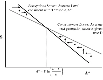
43 Therefore, we have immediately
Corollary One: S(A*) and E[S*] cross in one location. This produces the chart below
This leaves us with the very natural conclusion that if the members of a community guess
that college is more difficult than it really is fewer will work hard in high school and thus
fewer will go to higher education than would go under complete information. However, a
higher fraction of those who do go will return successfully than the members would have
predicted.
Perceptions Locus : Success Level consistent with Threshold A*
Consequences Locus: Average next generation success given true D
A
*
S
Intergenerational Dynamics
−
=
B C B D A* ln
44 Conversely, if the community members think that college is easier than it is than it is,
then too many will apply themselves in high school and too many will go on. However,
fewer will finish successfully than they expected.
Over time the community perceptions will converge towards the true value. This is
comforting both because it tends towards optimality and because it suggests that using
ones community as a source of information is over time helpful.
A key insight here is that if there is variation in community action and there is no
mechanism to bias the consequences a community will eventually converge on the truth.
Over time someone will breakout and try something new, in this case going to college.
That person will come back and influence the community. This in turn will encourage
more people to try and community perceptions will gradually move towards the truth.
Without parameterization, however, there is no way to tell how long this will take.
Bias, however, is a serious possibility in the community context. Community
composition is endogenous and more importantly life-choices and hence perceptions
influence community membership. If individuals select themselves into communities
based on common beliefs then the resulting actions of a community will be
systematically biased based on that belief and future generation will make incorrect
45 Ethnic prejudice may be example of beliefs about the state of nature that many readers
are familiar with. Ethnic prejudice seems to be strongly influenced by the community in
which one grew up. If a tight nit community believes that all people of a particular
ethnicity share some trait then the children raised in the community are likely to believe
that as well. This model of priors and endogenous community composition shows why
these beliefs persist so easily.
Individuals sort into communities on the basis of ethnicity. This is particularly true when
there are language barriers, as we might have imagined existed among immigrants to the
US in the 19th century. Therefore, the sorting process reduces the experiences necessary to update prejudices. Even more to the point, individuals who, for some idiosyncratic
reason, discard their prejudices are less likely to return to the community and affect the
priors of the next generation.
Young people growing up in the community do not know the state of nature. They have
no idea about the actual properties of ethnicities but they can deduce it from the behavior
of the adults. Through the sorting process their expose to adults who do not share
prejudice is limited and so the children rationally develop prejudice. Thus a system is
46 It is also immediately clear why negative false priors persist more strongly than positive
ones. Positive false priors encourage community mixing where the priors are then
updated. Negative false priors discourage it.
The sorting mechanism works similarly for beliefs about college. Adults who believe that
college is too difficult are concentrated by sorting and so the environment in which the
young students are raised is systematically biased. Thus, the young students rationally
conclude that college is too difficult.
How do Some Communities Remain Uneducated?
The above analysis presumed that all college grads returned to the community from
which the originated. However, suppose some fraction 1 – α left the community. That is,
after graduating from college they then joined a new community. For example, not all
towns have colleges and graduates might tend to stay in the town the graduated in and
become isolated from their original community.
In addition,n college graduates tend to have higher incomes than non grads and may
move into a more affluent neighborhood. The motivations will be considered later but for
47 If he moves to a new community then that graduates family line is replaced by a new
non-graduate family line.6
(3.1)
,
1 ,
,
1
( )
( ) 1
*
E[S*| A*,D, ]
*( *| )
( ) 0
*
i t A NK
D
i i t
i t
e
i
i
A
A
S
A D
i
A
A
N
δ α
δ
α
δ
− =
−
= ⇔
>
=
=
= ⇔
≤
∑
α passes through to yield:
(3.2)
E [S * | A *, D , ]
α
=
α
S
* ( * |
A
D
)
=
α
E [S *|A *,D ]
6
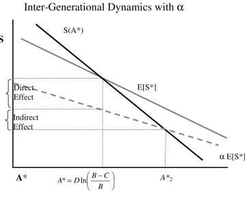
48 Simply put the fraction of expected graduate is reduced by the factor α.
The success rate in the community, however, is reduced by more than α. Not only do
fewer graduates return to the community, but the lower apparent success rate discourages
the next generation from trying. Rather than settling down to the true value of A* the
community settles on a higher value consistent with lower success. S(A*)
E[S*]
A
*
S
Inter-Generational Dynamics with
α
−
=
B C B D A* ln
α E[S*]
A*2 Direct
Effect
Indirect Effect
49 In this simple model community membership is binary. You are either in or out. There is
not possibility of being distantly connected or probabilistically connected. Therefore,
when individuals leave they no longer effect the estimation of the new generation. This
may not be that strong of an assumption.
We only have to assume that those who are partially disconnected from the community
are worse sources of information than those who are fully engaged. In that case if some
fraction β of graduates are partially disconnected, then there is an information loss of
equivalent of some α totally disconnected members.
There are two effects of α. There is the direct loss of graduates because some graduates
are ending up in another community. There is also the indirect loss of graduates because a
lower apparent success level discourages young students from working hard.
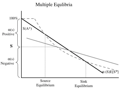
Interestingly, the size of the indirect effect is inversely proportional to the slope of S(A*).
If a wider range of A*s are consistent with a given range of success then the indirect
effect is increased. In equilibrium, the community must underestimate the success of
those who try by a factor of α. A shallow slope means that the tendency for agents to
underestimate the probability of success is low.
Therefore, a very high threshold and low success rate is necessary to pull underestimation