ODT Based Closure Model for Non-Premixed Combustion LES.

ABSTRACT

MILES, JEFFERY SCOTT. ODT Based Closure Model for Non-Premixed Combustion LES. (Under the direction of Dr. Tarek Echekki).

An LES closure method for turbulent non-premixed combustion using data from stand-alone ODT simulations is developed and validated. An ODT simulation provides a complete view of turbulent combustion including detailed chemistry within a single dimension through spatially (in 1D) and temporally resolved solutions for thermo chemical scalars and a stochastic description of turbulent advection. A unique closure technique removes the limitations associated with prescribed FDF distributions by using the resolved ODT statistics to construct joint scalar distributions needed for LES closure. These distributions are combined with other ODT statistics to construct closure tables for filtered variables such as density and chemical source terms. The tabulated closure follows the classical integration over state-space combining joint distributions with statistics from dependent variables. The temperature and mixture fraction are considered for this joint FDF as they can be combined to provide a complete view of the chemical and thermal state of the overall system within a non-premixed combustion problem. The ODT simulations are used to extract filtered and unfiltered correlations representing FDF distributions for each of the state-defining scalars; and kernel density functions are used to convert the sample datasets into smooth distributions that represent FDFs found within ODT statistics.

and stored in vector form with the “instantaneous” values for each term included in the un-closed set required in the LES domain. Model construction as well as the methods applied for data processing are described in addition to the design and application of LES closure. OpenFOAM, an open-source extensible CFD package, is used to implement the LES simulation needed to verify the proposed closure model.

ODT Based Closure Model for Non-Premixed Combustion LES

by

Jeffery Scott Miles

A dissertation submitted to the Graduate Faculty of North Carolina State University

in partial fulfillment of the requirements for the degree of

Doctor of Philosophy

Mechanical Engineering

Raleigh, North Carolina 2017

APPROVED BY:

_______________________________ _______________________________

Dr. Tarek Echekki Dr. Hong Luo

Committee Chair

_______________________________ _______________________________

DEDICATION

BIOGRAPHY

Jeffery Miles was born in Wooster, Ohio in 1970, but at a very young age, he moved south to North Carolina with his parents. After many different relocations and changes of address, Jeffery finally settled in Hickory, NC with his parents and 4 of his siblings. Jeffery gained a strong interest in computers at a very young age, and after high school chose to attend NC State, studying Computer Engineering. Even though Jeffery’s interest in computers centered more around the physics of the hardware, after graduation, he choose to pursue a career in software development. At the same time Jeffery was married to Twila whom he had met years before. Being newly married and working in software development, Jeffery and Twila set out to live a normal suburban lifestyle.

After working for more than 10 years in software development, Jeffery decided to try something different. With the help of two of his brothers, Jeffery built and raced a late-model stock car. Unfortunately, with the financials of the operation falling short, the racing business and his racing career came to an end, sooner than expected. All throughout the experience, Jeffery realized that science behind the race car was more interesting than the race car itself. Thus, after exiting his short racing career, Jeffery explored academic opportunities that align with automotive technologies. In the spring of 2005 Jeffery started a Master’s degree in mechanical engineering at NC State. After taking a few classes, combustion surfaced as a topic that interested Jeffery most. It was this interest combined with his remaining interest in computers that enticed him to purse a PhD in mechanical engineering focused on computation and combustion.

is 16 years old and in the 11th _{grade. Abigail is 17 years old in the 12}th _{grade. And Carl is 18}

years old in the 11th _{grade. Carl was the last addition to the family in that he was adopted from}

ACKNOWLEDGMENTS

I would like to thank my wife and kids for their many years of sacrifice and support during my academic pursuits. Each in their own way has provided encouragement and motivation for me to continue through all these years. I would also like to thank my mother, Dr. Gail Miles, and my father, Vern Miles for their wisdom and guidance both in my education and in my life. Thanks, also, to my brother Dr. Jeremy Miles who continues to motivate me by demonstrating what is possible, and to my other siblings for their companionship and encouragement.

A special thanks goes out to Dr. Tarek Echekki for the many years of advice and support. This effort would not have been possible without his dedication and patience helping me to advance every step of the way. I would also like to thank Dr. Hong Luo, Dr. Jack Edwards and Dr. Kevin Lyons for their willingness to serve on my committee. They have all been very encouraging and helpful in every aspect of my research. A particular thanks, also, goes to Dr. Phil Westmoreland who agreed on a very short notice to serve on my committee. His enthusiasm is contagious, and I appreciate his many efforts to make NC State University a good experience for all the students and faculty that he encounters.

TABLE OF CONTENTS

LIST OF TABLES ... ix

LIST OF FIGURES ... x

1 Introduction ... 1

1.1 Background and Motivation ... 1

1.2 Direct Numerical Simulation (DNS) ... 3

1.3 DNS Alternatives ... 7

1.4 State-Space Models ... 8

1.5 PDF Transport Method ... 11

1.6 Reduced Dimensional Models ... 13

1.7 Justification of ODT as a Closure Model ... 16

1.8 Research Objectives ... 19

1.9 Outline ... 20

2 LES Governing Equations ... 22

2.1 Background for Non-Premixed Combustion LES ... 22

2.2 Mixture Fraction ... 24

2.3 LES Momentum ... 28

2.4 Smagorinsky Model and Momentum Closure ... 30

2.5 LES Scalar Transport Equations ... 32

2.6 Density and Chemical Source Term ... 34

2.7 LES Closure with Filter Distribution Function ... 35

2.8 Variance Transport Equations ... 38

3 ODT Background and Formulation ... 42

3.1 Background ... 42

3.2 ODT Formulation ... 43

3.3 ODT and LEM Maps ... 47

3.4 Eddy Selection ... 50

3.5 Source Terms ... 53

3.6 Reduction of Dimensionality ... 55

3.7 Parameter Selection ... 56

4.3 Model Construction... 64

4.4 Kernel Density Function ... 66

4.5 FDF Construction using Kernel Density Function ... 68

4.6 Pre-Processing Raw ODT data ... 74

4.7 Post-Processing Raw ODT data ... 75

4.8 Final Integration ... 76

5 Piloted Jet Diffusion Flames ... 79

5.1 Sandia Flames ... 79

5.2 Extinction and Re-ignition in Sandia Flames ... 80

5.3 Piloted Burner Configuration ... 82

5.4 Available Experimental Data ... 85

5.5 Stand-alone ODT for non-premixed Sandia Flame ... 86

5.6 ODT Statistics ... 90

5.7 Kernel Density functions for ODT Distributions ... 108

5.8 Distribution Analysis ... 113

6 LES Results for Sandia Flame D ... 125

6.1 Flame D Introduction... 125

6.2 Mesh definition and Boundary Conditions ... 126

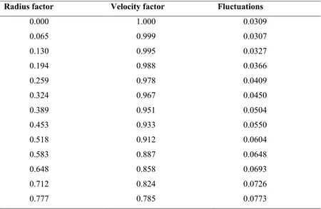
6.3 Flame D Velocity Profile ... 126

6.4 Flame D Cross Section ... 128

6.5 Flame D Axial Profiles ... 132

6.6 Flame D Radial Profiles ... 137

6.7 Flame D – State-Space Analysis ... 149

7 LES Results for Sandia Flame F ... 160

7.1 Flame F Introduction ... 160

7.2 Flame F Velocity profile ... 160

7.3 Flame F Cross Section... 162

7.4 Flame F Axial Profiles... 165

7.5 Flame F Radial Profiles ... 170

7.6 Flame F – State-Space ... 182

7.7 Variance and Scalar Dissipation ... 192

8.2 Model Performance and Accuracy ... 198

8.3 Challenges and Drawbacks ... 200

8.4 ODT-LES Model Variations ... 202

8.5 Necessary Improvements ... 204

8.6 Future Research and Suggested topics ... 205

REFERENCES ... 208

APPENDICES ... 215

Appendix A – LES solver using OpenFOAM ... 216

A1. Why Choose OpenFOAM ... 216

A2. “mixtureFractionFOAM” ... 217

A3. PIMPLE Method for solving Pressure and Velocity ... 218

A4. LES Density pressure dependence ... 220

A5. Boundary Conditions ... 221

A6. Heat transfer and Radiation Methods ... 223

A7. Scalar Variance Transport Equations ... 224

A8. Calculation of Temperature from Conservative Enthalpy ... 225

A9. Post Processing Analysis and Tools ... 227

Appendix B – MATLAB toolbox ... 228

B1. Introduction ... 228

B2. MATLAB Interpolation ... 228

B3. MATLAB FDF Construction ... 229

Appendix C – Additional Plots ... 230

C1. Sandia Flame D – Scalar Variance and Source Terms ... 230

C2. Sandia Flame F – Scalar Variance and Source Terms... 234

Appendix D – Statistics and Turbulent Combustion ... 238

D1. Statistical Background ... 238

D2. Histogram distributions ... 241

Appendix E – ODT Modeling: Additional information ... 243

E1. LES Filtering ... 243

E2. State Vector and Scalar Distribution Selection ... 244

Appendix F – Non-Premixed Flame Background ... 247

LIST OF TABLES

Table 4.1 FDF Construction Process... 73

Table 5.1 Initial Mass Fractions for pilot composition in piloted Methane Jet flame ... 85

Table 5.2 GRI 3.0 Reduced CH4 Chemical Mechanism ... 88

LIST OF FIGURES

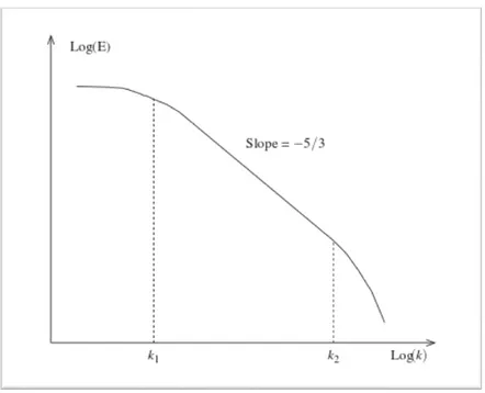
Figure 1.1 Log-log plot of Energy Spectra (Rebollo & Lewandowski, 2014) ... 17

Figure 3.1 Triplet Map transformation ... 50

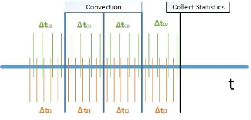
Figure 3.2 ODT Time steps... 52

Figure 4.1 Conditional PDF of temperature for Sandia Flame D, E, & F from experimental results (Barlow R. , 1999) ... 60

Figure 4.2 Conditional PDF of YH2O for Sandia Flame D, E, & F from experimental results (Barlow R. , 1999) ... 60

Figure 4.3 Conditional PDF of YOHfor Sandia Flame D, E, & F from experimental results (Barlow R. , 1999) ... 61

Figure 4.4 Conditional PDF of YCO for Sandia Flame D, E, & F from experimental results (Barlow R. , 1999) ... 61

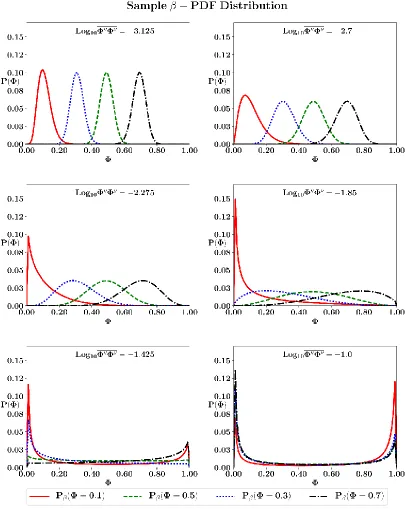
Figure 4.5 β-PDF Sample Distributions ... 62

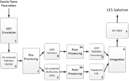
Figure 4.6 Process diagram illustrating construction of LES closure ... 66

Figure 4.7 Scalar Variance collections for Flame F... 71

Figure 4.8 Curve fit of Log10Z"Z" and Log10T"T" ... 72

Figure 5.1 Close-up of Sandia piloted flame burner (Barlow & Frank, 2007) ... 84

Figure 5.2 Density Contour plot conditioned on mixture fraction and temperature from un-processed ODT statistics for Flame F simulation ... 91

Figure 5.3 Rendered cross section view of ODT simulation for Flame F at in selective approximate downstream regions. ... 93

Figure 5.4 Axial profile of mixture fraction and temperature for ODT simulation of Flame F ... 95

Figure 5.5 Radial profiles of mixture fraction from ODT compared with from Barlow and Frank experiments at downstream distances of x/d=15,30,45 and 60 ... 96

Figure 5.6 Radial profiles of temperature from ODT compared with from Barlow and Frank experiments at downstream distances of x/d=15,30,45 and 60 ... 97

Figure 5.7 Comparison between ODT and experiments of conditional statistics for CH4 species mass fraction at downstream distances of x/d=15, x/d=30 and x/d=45 ... 100

Figure 5.8 Comparison between ODT and experiments of conditional statistics for O2 species mass fraction at downstream distances of x/d=15, x/d=30 and x/d=45 ... 101

Figure 5.9 Comparison between ODT and experiments of conditional statistics for H2O species mass fraction at downstream distances of x/d=15, x/d=30 and x/d=45 ... 102

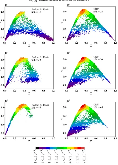
Figure 5.10 Comparison between ODT and experiments of conditional statistics for CO2 species mass fraction at downstream distances of x/d=15, x/d=30 and x/d=45 ... 103

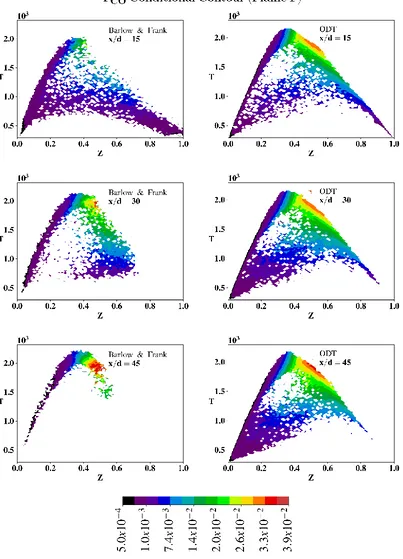
Figure 5.11 Comparison between ODT and experiments of conditional statistics for CO species mass fraction at downstream distances of x/d=15, x/d=30 and x/d=45 ... 104

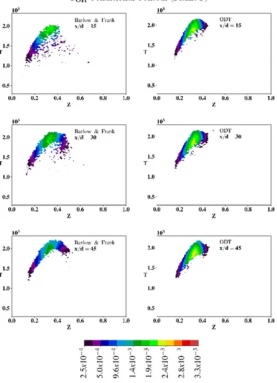
Figure 5.12 Comparison between ODT and experiments of conditional statistics for OH species mass fraction at downstream distances of x/d=15, x/d=30 and x/d=45 ... 105

Figure 5.15 Histogram and KDF distributions from ODT data at Z=0.1 and Z=0.5 for Flame D simulation. Note that the scale is different in the bottom two rows... 109 Figure 5.16 Histogram and KDF distributions from ODT data at Z=0.1 and Z=0.5 for Flame F simulation. Note that the scale is different in the bottom two rows. ... 110 Figure 5.17 Histogram and KDF distributions from ODT data at θT=0.1 and θT=0.5 for Flame D simulation. Note that the scale is different in the bottom two rows... 111 Figure 5.18 Histogram and KDF distributions from ODT data at θT=0.1 and θT=0.5 for Flame F simulation. Note that the scale is different in the bottom two rows. ... 112 Figure 5.19 Comparison of KDF with β-PDF at Z=0.1 and Z=0.5 for Flame D simulation. Note that the scale is different in the bottom two rows. ... 120 Figure 5.20 Comparison of KDF with β-PDF at Z=0.1 and Z=0.5 for Flame F simulation. Note that the scale is different in the bottom two rows. ... 121 Figure 5.21 Comparison of KDF with β-PDF at θT=0.1 and θT=0.5 for Flame D simulation. Note that the scale is different in the bottom two rows. ... 122 Figure 5.22 Comparison of KDF with β-PDF at θT=0.1 and θT=0.5 for Flame F simulation. Note that the scale is different in the bottom two rows. ... 123 Figure 6.1 Radial profile of axial velocity normalized by the centerline velocity U/UC ... 127 Figure 6.2 Temperature contour plot on 2D centerline cross section for Flame D. The greyscale line shows the stoichiometric mixture fraction. ... 129 Figure 6.3 H2 species mass fraction contour plot on 2D centerline cross section for Flame D.

The greyscale line shows the stoichiometric mixture fraction and the blue line shows the flame boundary. ... 130 Figure 6.4 CO2 species mass fraction contour plot on 2D centerline cross section for Flame

D. The greyscale line shows the stoichiometric mixture fraction and the blue line shows the flame boundary. ... 131 Figure 6.5 Axial Profiles of mixture fraction and temperature for Flame D ... 134 Figure 6.6 Axial Profiles of CH4, O2, H2O and CO2 Species Mass Fraction for Flame D . 135

Figure 6.7 Axial Profiles of CO, OH, H2 and NO Species Mass Fraction for Flame D ... 136

Figure 6.8 Radial profiles of mixture fraction at r/d = 2, 15, 30, 45, 60 ad 75 for Flame D ... 139 Figure 6.9 Radial profiles of Temperature at r/d = 2, 15, 30, 45, 60 and 75 for Flame D .. 140 Figure 6.10 Radial profile of CH4 species mass fraction at r/d = 2, 15, 30, 45, 60 and 75 for

Flame D ... 141 Figure 6.11 Radial profile of O2 species mass fraction at r/d = 2, 15, 30, 45, 60 and 75 for

Flame D ... 142 Figure 6.12 Radial profile of CO2 species mass fraction at r/d = 2, 15, 30, 45, 60 and 75 for

Flame D ... 143 Figure 6.13 Radial profiles of H2O mass fractions at r/d = 2, 15, 30, 45, 60 and 75 for Flame

Figure 6.17 Radial profile of NO species mass fraction at r/d = 2, 15, 30, 45, 60 and 75 for Flame D ... 148 Figure 6.18 Comparisons of conditional mean CH4 species mass fraction in state-space at

x/d=7.5, 15, 30, 45, 60 and 75 for Flame D. Note that “LES-ODT” is conditioned on Z, and “Barlow & Frank” is conditioned on Z. ... 152 Figure 6.19 Comparisons of conditional mean O2 species mass fraction in state-space at

x/d=7.5, 15, 30, 45, 60 and 75 for Flame D. Note that “LES-ODT” is conditioned on Z, and “Barlow & Frank” is conditioned on Z. ... 153 Figure 6.20 Comparisons of conditional mean H2O species mass fraction in state-space at

x/d=7.5, 15, 30, 45, 60 and 75 for Flame D. Note that “LES-ODT” is conditioned on Z, and “Barlow & Frank” is conditioned on Z. ... 154 Figure 6.21 Comparisons of conditional mean CO2 species mass fraction in state-space at

x/d=7.5, 15, 30, 45, 60 and 75 for Flame D. Note that “LES-ODT” is conditioned on Z, and “Barlow & Frank” is conditioned on Z. ... 155 Figure 6.22 Comparisons of conditional mean CO species mass fraction in state-space at x/d=7.5, 15, 30, 45, 60 and 75 for Flame D. Note that “LES-ODT” is conditioned on Z, and “Barlow & Frank” is conditioned on Z. ... 156 Figure 6.23 Comparisons of conditional mean NO species mass fraction in state-space at x/d=7.5, 15, 30, 45, 60 and 75 for Flame D. Note that “LES-ODT” is conditioned on Z, and “Barlow & Frank” is conditioned on Z. ... 157 Figure 6.24 Comparisons of conditional mean H2 species mass fraction in state-space at

x/d=7.5, 15, 30, 45, 60 and 75 for Flame D. Note that “LES-ODT” is conditioned on Z, and “Barlow & Frank” is conditioned on Z. ... 158 Figure 6.25 Comparisons of conditional mean NO species mass fraction in state-space at x/d=7.5, 15, 30, 45, 60 and 75 for Flame D. Note that “LES-ODT” is conditioned on Z, and “Barlow & Frank” is conditioned on Z. ... 159 Figure 7.1 Radial profile of axial velocity normalized by the centerline velocity U/UC ... 161 Figure 7.2 Temperature contour plot on 2D centerline cross section for Flame F. The greyscale line shows the stoichiometric mixture fraction. ... 163 Figure 7.3 H2 species mass fraction contour plot on 2D centerline cross section for Flame F.

The greyscale line shows the stoichiometric mixture fraction and the blue line is the outline of the flame. ... 164 Figure 7.4 CO2 species mass fraction contour plot on 2D centerline cross section for Flame

F. The greyscale line shows the stoichiometric mixture fraction and the blue line is the outline of the flame. ... 165 Figure 7.5 Axial Profiles of Mixture Fraction and Temperature for Flame F ... 167 Figure 7.6 Axial Profiles of CH4, O2, H2O and CO2 Species Mass Fraction for Flame F .. 168

Figure 7.7 Axial Profiles of CO, OH, H2 and NO Species Mass Fraction for Flame F... 169

Figure 7.11 Radial profiles of O2 mass fraction at downstream distances of x/d=2, 15, 30, 45

and 60 ... 175 Figure 7.12 Radial profiles of H2O mass fraction at downstream distances of x/d=2, 15, 30,

45 and 60 ... 176 Figure 7.13 Radial profiles of CO2 mass fraction at downstream distances of x/d=2, 15, 30,

45 and 60 ... 177 Figure 7.14 Radial profiles of OH mass fraction at downstream distances of x/d=2, 15, 30, 45 and 60 ... 178 Figure 7.15 Radial profiles of CO mass fraction at downstream distances of x/d=2, 15, 30, 45 and 60 ... 179 Figure 7.16 Radial profiles of H2 mass fraction at downstream distances of x/d=2, 15, 30, 45

and 60 ... 180 Figure 7.17 Radial profiles of NO mass fraction at downstream distances of x/d=2, 15, 30, 45 and 60 ... 181 Figure 7.18 Comparisons of conditional mean CH4 species mass fraction in state-space at

x/d=7.5, 15, 30, 45, 60 and 75 for Flame F. Note that “LES-ODT” is conditioned on Z, and “Barlow” is conditioned on Z. ... 184 Figure 7.19 Comparisons of conditional mean O2 species mass fraction in state-space at

x/d=7.5, 15, 30, 45, 60 and 75 for Flame F. Note that “LES-ODT” is conditioned on Z, and “Barlow” is conditioned on Z. ... 185 Figure 7.20 Comparisons of conditional mean H2O species mass fraction in state-space at

x/d=7.5, 15, 30, 45, 60 and 75 for Flame F. Note that “LES-ODT” is conditioned on Z, and “Barlow” is conditioned on Z. ... 186 Figure 7.21 Comparisons of conditional mean CO2 species mass fraction in state-space at

x/d=7.5, 15, 30, 45, 60 and 75 for Flame F. Note that “LES-ODT” is conditioned on Z, and “Barlow” is conditioned on Z. ... 187 Figure 7.22 Comparisons of conditional mean OH species mass fraction in state-space at x/d=7.5, 15, 30, 45, 60 and 75 for Flame F. Note that “LES-ODT” is conditioned on Z, and “Barlow” is conditioned on Z. ... 188 Figure 7.23 Comparisons of conditional mean CO species mass fraction in state-space at x/d=7.5, 15, 30, 45, 60 and 75 for Flame F. Note that “LES-ODT” is conditioned on Z, and “Barlow” is conditioned on Z. ... 189 Figure 7.24 Comparisons of conditional mean H2 species mass fraction in state-space at

1

Introduction

1.1

Background and Motivation

Never before has the study of power generation and heating systems fueled by combustion of fossil fuels and bio-fuels been more important. Due to the never-ending threat of global warming and competition from alternative energy sources, efficiency and environmental conservation continue to grow as important factors in designing and applying these systems. A complementary concept that many times enhances the combustion process is turbulence. Making the overall system more efficient and effective, turbulence provides a mechanism by which available kinetic energy is leveraged in the mixing process. Unfortunately, this increased efficiency always comes with a price. Adding turbulence to a reacting flow enhances mixing, but it also increases the complexity and instability. Turbulence tends to affect the reaction mechanism just as system changes due to combustion affect the turbulent flow characteristics. The inability to capture this relationship completely can lead to inefficient system designs that generate more pollutants or waste more fuel. Modern research on the subject of turbulent combustion continues to focus on the interactions between turbulence and reacting flows to understand and leverage the benefits better while avoiding the pitfalls.

setting up and running computer models. Experimental studies are necessary to understand the science governing a model, but long term results are best obtained from re-application of computer simulations which can be adjusted to fit requirements specific to a given domain. In general, there is an inverse relation between the degree of empiricism included in a model and the versatility of its application. Simulations that contain a higher degree of empiricism tend to work best for environments and domains which match that of the original design. Models that are more true to the physics while accounting for the numerical limits have a wider scope of application. Unfortunately, the complexity of turbulent combustions makes the balance between versatility and empiricism even more important. As a result, numerical studies which focus on turbulent combustion continue to be important and draw much attention within the energy research community.

challenge then for any computer model is to capture the necessary time scales as well as the important length scales simultaneously using a reasonable amount of resources while also staying within a reasonable degree of accuracy.

1.2

Direct Numerical Simulation (DNS)

To be effective, a numerical solution designed to operate with a computer must solve the given problem efficiently while also containing the discretization and numerical errors. Due to the large differences in spatial and temporal scales mentioned above, a discrete solution which solves the differential equations governing a turbulent reacting system directly must operate within an extremely fine grid capable of capturing all the length scales. In addition, extremely small time steps may be required to capture all the time scales that are present. Direct solutions to the widely accepted Navier-Stokes equations governing a turbulent fluid flows are generally named Direct Numerical Solutions (DNS) due to the lack of simplifying models or assumptions. These solutions are strapped with scale and complexity limitations due to the many factors mentioned above. As discussed in (Veynante & Poinsot, 2005), the number of grid points needed to represent a turbulent flow problem properly at a given Reynolds number limit is proportional to the ratio of the largest scales to the smallest scales:

[𝑙

𝜂< 𝑁]. A good domain definition must then balance the limitations on the size of the domain,

limitations to the Reynolds number and limitations on the number of grid points.

𝑅𝑒_𝑡< 𝑁4⁄3 (1.1)

of reacting flows reveal that the grid must be small enough to capture the reaction mechanism within a given residence time, meaning the inner portion of the domain must be fine enough to resolve all of the flame elements represented in the regions surrounding a flame. As a result, limitations for a numerical simulation of a turbulent reacting flow can be expressed as the ratio of the largest scale in the domain to the flame thickness in conjunction with the ratio of the overall number of grid points and the inner region size needed to capture the flame. With Q representing the number of grid points necessary to capture the important parts of a flame structure, this limitation relates the product of the turbulent Reynolds number and the Damköhler number to the square of inner and outer portions of the grid (Veynante & Poinsot, 2005).

𝑅𝑒𝑡𝐷𝑎 < ( 𝑁 𝑄)

2

(1.2)

The term 𝑅𝑒𝑡𝐷𝑎 is an expression which captures the combination of fluid motion and the speed

of the small-scale processes. 𝑁

𝑄 is an expression which illustrates the cost of simultaneously capturing the large regions of the domain while also representing the physics occurring in the smaller portions. Eq. (1.2) explains the limitations of what DNS studies can accomplish with the allotted computational resources.

iteration of a computation. This complexity is generally not feasible for domains of any significant size. Intrinsic Low Dimensional Manifold (IDLM) is used to reduce the overall picture of a more detailed mechanism. This procedure separates the reactive species, focusing on the ones with slower chemical- reaction time scales. Requiring fewer species to reach a solution facilitates a more tractable solution, however, neglecting the species with faster time scales limits the range of flame conditions that can be modeled (Maas & Pope, 1992). IDLM works best with reactions that always progress to equilibrium, but it falls short in scenarios such as extinction and re-ignition where the faster reaction rates are affected by the turbulent characteristics. Another promising method designed to handle the complex chemistry needed for reactive DNS studies is the In Situ Tabulation (ISAT) method, where the chemical source values at a given state are stored in a dynamically constructed table. With the ISAT procedure, the state vector is represented using a binary tree, and the chemical source terms are stored for recently performed calculations (Pope S. , 1997). Later in the computation, when the same state conditions are encountered again, the calculations can be skipped in lieu of a table lookup. As expected, this procedure works best with problems where local equilibria are predominant. While these methods provide excellent options for capturing more detailed chemical compositions, they come with a cost: the limitations resulting from assumptions and bounding conditions. As stated before, each method tends to improve the solution capacity in one way by restricting it in others.

1.3

DNS Alternatives

above, the complex relationship between turbulent motion and combustion is difficult to capture with any type of numerical solution. This difficulty is especially true within reduced scale mechanisms that cut out the very portions of the solution where the combustion is occurring. For this reason, many different methods have been investigated to solve this part of the closure problem. Some have persisted, some have not.

Several major approaches have been developed for resolving the closure problem associated with RANS and LES solutions to turbulent reacting flows. The majority of these methods were first developed for RANS and then later extended to LES. The extension is natural because, even though RANS and LES differ in how the reduction is defined, the resolved equations for each have similar forms. The differences stem from contrasts between an averaging function and a filtering function, which cannot be taken lightly. As a result, comparisons between each model must consider the necessary assumptions closely before expanding to more general problem spaces. Many of these closure methods fall into one of three main categories: sample space, PDF transport, and reduced dimensional stochastic models. While different in construction and formulation, each method has a similar object of representing the information residing in the scales smaller than the LES grid with a tractable, accurate solution. Each method is challenged by issues specific to the particular formulation, and how these problems are handled determines the resulting success.

1.4

State-Space Models

conservative and reacting scalar. For flows that exhibit extinction and re-ignition, the β-PDF is not able to capture all the scalar distributions present accurately. Finally, the scale separation assumption limits the problem to a small class of flames where the flames are thinner than the smallest scales in the flow. Despite all these challenges, the flamelet model is still widely used and continues to draw attention in studies applying LES to represent turbulent reactive flows numerically. This popularity is mostly due to the simplicity and the wide spread adoption among commercial CFD codes.

assessment with a study on how sensitive the CMC methods are to the LES grid. With the scalar dissipation being an exception, all of the conditional variables appeared to be insensitive to grid resolution. This finding is consistent with other known issues in dealing with the filtered scalar dissipation term.

1.5

PDF Transport Method

with the turbulent fluctuations and how they affect the distribution. This challenge is evident in the expansion and development of the many different mixing models used to close the turbulent portions of the PDF transport equation (S.Viswanathan, Wang, & Pope, 2011). The most distinct challenge with PDF methods has to do with the computational cost of a direct solution to the PDF transport equation. The computational cost of a direct solution is higher than feasible because the joint PDF is based on a significant number of dimensions making it intractable in current computational space. Researchers instead have turned to stochastic methods such as the Lagrangian Monte Carlo method to solve the PDF transport equation in the spatial domain (Colucci, Jaberi, Givi, & Pope, 1998). While this method is good, a strategy is needed to manage the errors that result from using a finite number of particles within the Lagrangian transport process. As particles are transported within the solution, the overall state is a combination of each of the particles within a computational cell, which means that empty cells are a possibility. This situation must be avoided because it would represent a discontinuity.

between averaging and filtering. Needless to say, the solution methods must still take advantage of complex stochastic methods to close the final transport equations.

One novel application combines the physics represented in the laminar flamelet with the PDF obtained through transported distributions (Wang & Chen, 2005). This method applies the flamelet concept as above, but the PDFs used to calculate the filtered/averaged quantities are those transported using the Monte-Carlo solution for the joint scalar/velocity PDF. This approach simplifies the PDF transport equations by only including the PDF for the mixture fraction and the TKE transfer rate. Assuming that there is enough information in the fluctuations of these two terms to account for both scalar mixing and turbulent motion, these transported PDFs combined with the flamelet models are all that is required to close the LES solution. Historically, the filtered/averaged scalar dissipation rate has been difficult to describe, leading to the inclusion of an assumed PDF for the scalar dissipation rate (Pitsch & Steiner, 2000). Alternatively, this Flamelet-PDF method proposes an algorithm to construct the scalar dissipation rate distribution from the mixture fraction and the TKE transfer rate which are resolved via the PDF transport method. Unfortunately, the issues associated with Monte-Carlo transport equation solvers are still challenges in addition to the limitations due to the scale separation assumption.

1.6

Reduced Dimensional Models

dimensional problem, the stirring that results from turbulence must be simulated via a stochastic model. Both (Linear Eddy Model) LEM and (One-Dimensional Turbulence) ODT use the “maps” concept to simulate stirring events which discretely model turbulent flow patterns. These mapping events are dependent on a probability of selecting a random location at a given time with a likely size and shape (Kerstein A. , 1999). Both simulations are driven by an eddy rate that determines this probability; however, they differ in the complexity of the rate calculation. LEM uses empirically determined constants while ODT uses a coupling based on transported flow properties. Realizations from LEM and ODT solutions generally contain the composition detail for a given state which also implicitly includes all of the necessary statistical information. Closure methods are at liberty to choose how to capture the statistical information and provide a working model accordingly. Early usage of these methods uses a prescribed probability distribution to determine the likelihood of a given filtered state, but recent developments have taken advantage of the implicit distributions resulting from PDF’s condition on filtered state variables (Ranganath & Echekki, 2008; Sankaran, Drozda, & Oefelein, 2009).

methods, implementations that support detailed chemistry models have potential limitations in the available computational infrastructure needed to provide an ideal performance.

Considering the methods discussed thus far, it is apparent that continued research is valuable to making each approach more robust and effective. Also, because these methods are mature enough to warrant industrial use, they frequently appear as extensions to commercial software. Regardless of adaptation, each method can benefit from improvements and enhancements to the models and implementations. Many of the recent advancements with these models include solutions for new problem spaces that have yet to be solved, and during these implementations, the new findings are then used to enhance the models further. This statement is true mostly for flamelet and PDF transport models where the methods are very mature and tend to be seen as the better choices for select problem domains. On the other hand, low-dimensional models have yet to reach all of the potential available. Thus, in addition to research expanding the use of low dimensional models, researchers continue to explore the untapped information that can be extracted from these simulations.

choice implementations; however, tabulation methods still have their place in future developments. Stand-alone methods offer a high degree of runtime simplicity with a smaller up-front investment, and they have the ability to interchange reaction mechanisms with little changes to the integrated model. Much of the new research required for coupled solutions involves the coupling mechanism between LES and ODT and improved efficiencies in the implementation. The interchange of information between these two solutions is paramount to the effectiveness of the method. Variables in the LES space require increased resolution, while information obtained from ODT requires reduced resolution. The difference introduces unnecessary error which may affect the outcome. In contrast, within the tabulation space, the biggest concern is finding an effective and efficient mechanism to represent the statistical nature of the solution. These methods either encapsulate the statistics and the spatial information within the same constructs, or they separate the statistics and combine the model via an integration step. Accurately representing the statistical nature is essential to predicting unresolved quantities within highly turbulent reactive flows. With the many layers of complex information, modeling the statistics can be quite difficult otherwise.

1.7

Justification of ODT as a Closure Model

from the largest scale to the smallest. Reviewing a log of energy (log(E(k))) vs. wave number k plot reveals that the wave number increases linearly as the energy is transferred downward in the inertial range. This energy is then dissipated sharply beyond a certain wave number at or below the Kolmogorov scale.

The general idea behind the mixing model applied in LEM is that the transfer of information across the inertial subrange is accomplished by incrementally increasing the wave number on which the data distribution representing transported scalars resides. By matching

the information within the added frequencies to the linear effects of a turbulent eddy, LEM can capture both the motion and signal characteristics of turbulence in a single operation.

At the core of an LEM model is the triplet map, which is a very simple process that captures a linear representation of an eddy. It is a two-step process that involves both compression and rotation. The compression is accomplished by increasing the slope of the data and therefore reducing the length portion of the output signal. The modeling of rotation is achieved by flipping one-third of the data within the mapped region. The triplet map is thus a linear mechanism to represent the motion and statistical nature of the turbulent flow. The important thing to note is that the maps have the same effect as a turbulent eddy: they add additional frequencies, thereby reducing which length scales are more relevant in the modeled space. Over time, the length scales carrying important information are reduced to the smallest layer matching that of the molecular processes.

A significant limitation with a 1D solution involves the orientation of the chosen domain. For many of the flows studied using ODT and LEM, the chosen domain is a cross section perpendicular to the dominant velocity pattern. For problem domains that involve a symmetrical or axisymmetric shear layer, this positioning of the 1D domain works quite well. (Echekki T. , Kerstein, Dreeben, & Chen, 2001) provide several examples where a time-marching ODT solution for a symmetric channel or an axisymmetric jet can perform as well as a DNS solution given the proper boundary conditions. Unfortunately, in regions where the shear layer isn’t as well defined, selecting the placement of the 1D domain and the boundaries can be much more difficult. To overcome this challenge, models must account for more domains simultaneously, which is more difficult mathematically and computationally. In response to these challenges, coupled solutions model LES sub-grids via interlaced ODT domain. This type of approach enables application to a variety of domains, and expanding the number of applicable domains is vital to the growth of ODT research. Nonetheless, research continues to advance the traditional prescribed domain method because of its efficiency and reduced overhead.

1.8

Research Objectives

correlations extracted between filtered and unfiltered terms are a perfect source to build a filter density function. These constructed distributions provide a more realistic view of what PDFs are needed to build a state-based closure model that is an improvement over prescribed PDFs, such as the β-PDF. It follows that a stand-alone closure model can be built naturally by integrating over the ODT state-space with the extracted distributions. This combination of two separate aspects of the flow essentially reconstructs what was already present in the ODT solution, but in a form that is accessible via a filtered state vector. Models assembled in this fashion are validated via a known flow problems that have experimental data available for comparison. The ODT stand-alone model is validated using an LES solver built with OpenFOAM to simulate the Sandia piloted jet diffusion Flames.

1.9

Outline

2

LES Governing Equations

2.1

Background for Non-Premixed Combustion LES

The derivation of LES governing equations starts with the resolved instantaneous conservation equations for a reacting mixture. Traditionally, Eulerian solutions to fluid problems start with the 3D formulation of the Navier-Stokes equations for compressible fluids (Peters, 2000). Within a closed aggregate system, where the fluid is treated as a statistical collection of particles, the Navier-Stokes equations describe the conservation of three key characteristics of the system: mass, momentum, and energy (Acheson, 1990). Conservation of mass captures the chemical and physical state of the fluid, which is comprised of a mixture of species components. The species component vector describes the individual species contributing to the mixture and provides access to many of the fluid properties such as viscosity, diffusivity and density. Momentum captures the results of a mass in motion. In the case of a mixture, momentum is the effect carried with the moving sum of all the transported species. The momentum equation is simplified by viewing the mixture as a sum of all the parts, which is the fluid density. Combining the fluid density with the directional velocity of the bulk fluid (𝜌𝑢_𝑖) gives a single view of the fluid momentum. Finally, the conservation of energy equation captures the potential, kinetic, thermal, and chemical energy within a system. For chemically reactive systems, these contributions all play a very complex role in the overall system.

𝜕𝜌 𝜕𝑡 +

𝜕𝜌𝑢𝑖

𝜕𝑥_𝑖 = 0 (2.1)

𝜕𝜌𝑌_𝑘 𝜕𝑡 + 𝜕𝜌𝑢_𝑖𝑌_𝑘 𝜕𝑥_𝑖 = 𝜕 𝜕𝑥_𝑖(𝜌𝐷𝑘 𝜕𝑌_𝑘

𝜕𝑥_𝑖) + 𝜔𝑘̇ (2.2)

𝜕𝜌𝑢_𝑗 𝜕𝑡 + 𝜕𝜌𝑢_𝑖𝑢_𝑗 𝜕𝑥𝑖 = 𝜕 𝜕𝑥𝑖 (𝜏𝑖𝑗) − 𝜕𝑃 𝜕𝑥𝑗 (2.3) 𝜕𝜌ℎ𝑡 𝜕𝑡 + 𝜕𝜌𝑢𝑖ℎ𝑡 𝜕𝑥_𝑖 − 𝜕𝑝 𝜕𝑡 = 𝜕 𝜕𝑥𝑖 (𝑢𝑗𝜏𝑖𝑗) − 𝜕𝑞_𝑖 𝜕𝑥𝑖 + ∑ 𝜌𝑌𝑘𝑓𝑖𝑘∙ (𝑢𝑖+ 𝑉𝑖𝑘) 𝑁 𝑘=1 + 𝑸̇ (2.4)

In Eq. (2.2), 𝐷_𝑘 is the diffusion coefficient of species k into the rest of the mixture, and 𝜔_𝑘̇ is

the change in species k due to chemical reactions. 𝜕

𝜕𝑥𝑖(𝜏𝑖𝑗) represents changes to the

momentum due the viscous forces within the fluid, and for Newtonian fluids this term can be written in terms of a stress tensor which captures changes in the fluid due to shear forces (Kuo, 2005).

𝜕

𝜕𝑥_𝑖(𝜏𝑖𝑗) = 𝜕

𝜕𝑥_𝑖(2𝜇 (𝑆𝑖𝑗 − 1

3𝛿𝑖𝑗𝑆𝑘𝑘)) (2.5)

where

𝑆_𝑖𝑗 =1 2(

𝜕𝑢𝑖 𝜕𝑥_𝑗 +

𝜕𝑢_𝑗

𝜕𝑥_𝑖) (2.6)

Here, 𝜇 is the fluid viscosity, 𝛿_𝑖𝑗 is the Kronecker delta, 𝑆_𝑖𝑗 is fluid stress tensor, and 𝑆_𝑘𝑘 is the

and chemical changes in the fluid. In Eq. (2.4), 𝜕

𝜕𝑥𝑖(𝑢𝑗𝜏𝑖𝑗) is the dissipation due to viscous

forces, ∑𝑁𝑘=1𝜌𝑌𝑘𝑓𝑖𝑘∙ (𝑢𝑖+ 𝑉𝑖𝑘) is the result of body forces within the fluid, and 𝑸̇ is the heat

added to the system. 𝜕𝑞𝑖

𝜕𝑥𝑖 contains changes due to heat transfer which include conduction,

diffusion and Dufour effects. A key aspect of the LES method that makes the governing equations more robust than the corresponding DNS method is the application of a spatial filter. This filter limits the solution to a manageable range of data frequencies, but it also adds additional complexities to the solution. In order to minimize these complexities several steps are taken to simplify Eqs. (2.1) through (2.4) prior to filtering.

2.2

Mixture Fraction

fraction can be expressed in terms of fuel and oxidizer stream mass fractions, but for complex mixtures using elemental mixture fractions works best.

Equation (2.7) was introduced in (Bilger, 1988) as a universal expression for mixture fraction. Being comprised of all of the elemental mixture fractions, this equation is valid for all mixture compositions regardless of the number of species.

𝑍 =

2(𝑍𝐶− 𝑍𝐶.𝑂) 𝑊_𝐶

⁄ +

1

2(𝑍𝐻− 𝑍𝐻.𝑂) 𝑊_𝐻

⁄ ₊(𝑍𝑂− 𝑍𝑂.𝑂) 𝑊_𝑂 ⁄

2(𝑍_𝐶,𝑓− 𝑍_𝐶.𝑂) 𝑊_𝐶

⁄ ₊

1

2 (𝑍𝐻,𝑓− 𝑍𝐻.𝑂) 𝑊_𝐻

⁄ ₊(𝑍𝑂,𝑓− 𝑍𝑂.𝑂) 𝑊_𝑂 ⁄

(2.7)

In Eq. (2.7), the elemental mixture fractions are the sum of the contributions from each of the mass fractions present that contain the element.

𝑍𝑗 = ∑ 𝑎_𝑖𝑗𝑀_𝑗 𝑀𝑖 𝑌𝑖 𝑁 𝑖=1 (2.8)

Using the expression in Eq. (2.7) to reduce Eq. (2.2) to a mixture fraction transport equation can be quite difficult. To simplify this process, the mixture fraction defined via elemental mixture fractions can be reduced to an equation in terms of fuel and oxidizer mass fractions. This transformation starts with a theoretical reaction in terms of fuel and oxidizer leading to a product.

𝐹 + 𝑂 = 𝑃 (2.9)

Considering 𝐶𝐻₄ and 𝑂₂ as the fuel and oxidizer respectively, the above expression can be written as a single step methane + oxygen reaction.

The mass fractions from the fuel-oxidizer equation -- Eq. (2.9) -- and the methane reaction – Eq. (2.10) -- are defined as 𝑌𝐹 = 𝑌𝐶𝐻4 and 𝑌𝑂 = 𝑌𝑂2. With these definitions, the elemental

mixture fractions can also be expressed in terms of a fuel and oxidizer mass fraction: 𝑍𝐶 = 𝑀𝐶𝑌𝐹

𝑀𝐹 , 𝑍𝐻 =

4𝑀𝐻𝑌𝐹

𝑀𝐹 and 𝑍𝑂 =

4𝑀𝑂𝑌𝑂

𝑀𝑂 . To continue, a single conserved scalar, 𝛽 in terms of

𝑍_𝐶, 𝑍_𝐻 and 𝑍_𝑂 is defined.

𝛽 = 𝑍𝐶 𝑀_𝐶+

𝑍_𝐻 4𝑀_𝐻−

𝑍_𝑂

2𝑀_𝑂 (2.11)

After substituting the expressions for elemental mass fraction, 𝛽 can be expressed in terms of species mass fractions.

𝛽 = 𝑌𝐹 𝑀𝐹

+ 𝑌𝐹 𝑀𝐹

− 2𝑌𝑂 𝑀𝑂

𝛽 = 2𝑌𝐹 𝑀𝐹

− 2𝑌𝑂 𝑀𝑂

𝛽 = 𝑌𝐹− 𝑀_𝐹 𝑀_𝑂 𝑌𝑂

𝛽 = 2𝑌_𝐹− 2 (𝐹 𝑂)𝑠𝑡

𝑌_𝑂 (2.12)

The solution mixture fraction is defined in terms of 𝛽 for the mixture, 𝛽 for the fuel stream and 𝛽 for the oxidizer stream.

𝑍 = 𝛽 − 𝛽𝑂

𝛽_𝑭− 𝛽_𝑶 (2.13)

𝑍 =

2𝑌𝐹− 2 (𝐹 _{𝑂 )}

𝑠𝑡𝑌𝑂− (−2 ( 𝐹 𝑂 )𝑠𝑡)

2 − (−2 (𝐹 _{𝑂 )} 𝑠𝑡)

(2.14)

If (𝐹

𝑂)_𝑠𝑡 = 1 as before, then Eq. (2.14) can be simplified to the following.

𝑍 =2𝑌𝐹− 2𝑌𝑂+ 2

2 + 2 =

1

2[1 + 𝑌𝐹− 𝑌𝑂] (2.15)

The final expression, Eq. (2.15) is then be combined with the species transport Eq. (2.2) to form an equation for the mixture fraction.

𝜕𝜌𝑌_𝐹 𝜕𝑡 − 𝜕𝜌𝑌_𝑂 𝜕𝑡 + 𝜕𝜌𝑢_𝑗𝑌_𝐹 𝜕𝑥𝑗 −𝜕𝜌𝑢𝑗𝑌𝑂 𝜕𝑥𝑗 = 𝜕 𝜕𝑥_𝑗(𝜌𝐷𝑘 𝜕 𝜕𝑥_𝑗𝑌𝐹) − 𝜕 𝜕𝑥_𝑗(𝜌𝐷𝑘 𝜕 𝜕𝑥_𝑗𝑌𝑂) + 𝜔𝐹 − 𝜔_𝑂 (2.16)

In Eq. (2.16) the sum of the source terms are equal to zero (𝜔_𝐹 = 𝜔_𝑂), the derivative of a constant is equal to zero, and the species diffusion coefficients are assumed equal. Thus, the transport equation for the mixture fraction reduces to the following.

𝜕𝜌𝑍 𝜕𝑡 + 𝜕𝜌𝑢_𝑗𝑍 𝜕𝑥_𝑗 = 𝜕 𝜕𝑥_𝑗(𝜌𝐷𝑧 𝜕

𝜕𝑥_𝑗𝑍) (2.17)

2.3

LES Momentum

The transformation of the conservation equations into the LES domain requires application of a spatial filter to cut off the high-frequency (or small-scale) contributions (McDonough, 2007). This filtering process appears as an integration, applying a filter function over the spatial domain.

𝛹̅ = ∫ 𝐺(𝑥𝑖 − 𝜉)𝛹(𝜉)𝑑𝜉 (2.18)

While any symmetrical filter kernel G will work, many times a Gaussian or Box filter is used for simplicity. The filtering operation is different from the averaging function used with RANS, but the two operations share enough properties to render similar governing equations. Namely, because both are expressed as integrals, both share the distributed property allowing each contribution to be filtered separately. The filtered version of Eq. (2.3) is listed below.

𝜕𝜌𝑢̅̅̅̅̅_𝑖 𝜕𝑡 + 𝜕𝜌𝑢̅̅̅̅̅̅̅𝑗𝑢𝑖 𝜕𝑥_𝑗 = 𝜕 𝜕𝑥_𝑗(𝜏̅̅̅̅̅̅ −𝑖𝑗) 𝜕𝑃̅

𝜕𝑥_𝑖 (2.19)

Filtering a convolutions such as 𝑢_𝑗𝑢_𝑖 is also similar to the averaging function because the term

𝜕𝜌𝑢̅̅̅̅̅̅̅̅𝑗𝑢𝑖

𝜕𝑥𝑗 results in a complex set of individual contributions when decomposed. The filtered

advection term is not tractable; thus, further analysis is required to obtain an equation which is able to be solved. Again, much like the RANS averaging, the density can be separated using a averaged filtering which separates the filtered density from the filtered product. Favre-averaged filtering involves separating the filtered density from the filtered product by dividing the filtered product with the filtered density.

Equation (2.20) is simplified by expressing the integral in terms of the filter notation.

𝛹̃ =𝜌𝛹(𝜉)̅̅̅̅̅̅̅̅

𝜌̅ (2.21)

A simple manipulation of Eq. (2.21) leads to the natural expression 𝜌̅𝛹̃ = 𝜌𝛹(𝜉)̅̅̅̅̅̅̅̅ _{which can} be substituted into Eq. (2.19) resulting in the following form for the momentum equation.

𝜕𝜌̅𝑢̃𝑖 𝜕𝑡 + 𝜕𝜌̅𝑢̃_𝑗𝑢_𝑖 𝜕𝑥_𝑗 = 𝜕 𝜕𝑥_𝑗(𝜏̅̅̅̅̅̅ −𝑖𝑗) 𝜕𝑃̅

𝜕𝑥_𝑖 (2.22)

The next step is to express 𝑢̃𝑗𝑢𝑖 in terms that can be explained through alternate means. The

term 𝑢̃_𝑗𝑢_𝑖 can be expanded to 𝑢̃ = 𝑢_𝑗𝑢_𝑖 ̃ − 𝑢_𝑗𝑢_𝑖 ̃ 𝑢_𝑗̃ + 𝑢_𝑖 ̃ 𝑢_𝑗̃_𝑖 which can then be substituted into

Eq. (2.22). 𝜕𝜌̅𝑢̃𝑖 𝜕𝑡 + 𝜕𝜌̅𝑢̃ 𝑢_𝑗̃_𝑖 𝜕𝑥_𝑗 = − 𝜕 𝜕𝑥_𝑗𝜌̅(𝑢̃ − 𝑢𝑗𝑢𝑖 ̃ 𝑢𝑗̃ ) +𝑖 𝜕 𝜕𝑥_𝑗(𝜏̅̅̅̅̅̅ −𝑖𝑗) 𝜕𝑃̅

𝜕𝑥_𝑖 (2.23)

The expression (𝑢̃ − 𝑢𝑗𝑢𝑖 ̃ 𝑢𝑗̃ ) is formally termed the sub-grid stress, and it represents the 𝑖 viscous dissipation of turbulent energy at scales below the filter size. Without a direct solution, this expression must be modeled such that it can be resolved with known quantities.

The sub-grid stress, 𝜌(𝑢̃ − 𝑢𝑗𝑢𝑖 ̃ 𝑢𝑗̃ ), is assumed to follow a dissipative character and 𝑖 can be modeled in terms of the large scale strain-rate. More formally, this can be expressed using an SGS-eddy viscosity (Ferziger, 1996):

𝜌̅(𝑢̃ − 𝑢_𝑗𝑢_𝑖 ̃ 𝑢_𝑗̃ ) ≡ Τ_𝑖 ̃ ≅ −2𝜇_{𝑖𝑗 𝑆𝐺𝑆}𝑆̃_𝑖𝑗 (2.24)

where Τ̃𝑖𝑗 represents the eddy-viscosity SGS stress term, 𝜇𝑆𝐺𝑆 is the perceived viscosity due to

In a numerical sense, the SGS stress provides the numerical dissipation needed to make a coarse-grained solution more stable. The SGS-eddy viscosity 𝜇_𝑆𝐺𝑆 must relate the available energy to the possible dissipative character of the flow, and thus it must be modeled using concepts relating the available flow energy to a viscosity. If all the available energy is assumed to be dissipated via this eddy viscosity then, the SGS viscosity can be modeled in direct relation to the magnitude of the shear stress.

|𝑆̃| = √2𝑆̃𝑆_𝑖𝑗̃_𝑖𝑗 (2.25)

What remains is an expression that captures the size of the filter used to remove this lost information. As seen in the next section, including the LES filter size in the definition of the SGS viscosity quantifies the detail lost.

2.4

Smagorinsky Model and Momentum Closure

In the 19th _{Century, Boussinesq proposed that the turbulent stress seen in Eq. (2.24) is}

proportional to the velocity gradient, much like the stresses seen in laminar flow. This idea likens the eddy viscosity to the mixing length, which is related to the magnitude of the stress tensor. (Smagorinsky, 1963) formalized this theory for LES by considering that the filter width is also related to the mixing length, thus contributing to the exhibited turbulent stresses. With these ideas, the SGS viscosity is considered to be proportional to the magnitude of the shear stress and the filter width (McDonough, 2007).

𝜇_𝑆𝐺𝑆 = 2𝐶_𝑠2Δ2|𝑆̃| (2.26)

performs reasonably well in free-flowing jets with known levels of turbulence. As a result, this approach is a decent choice for a round jet surrounded by a free stream. The dissipation issues and flexibility can be relaxed with a formulation that determines 𝐶𝑠 dynamically, but this approach adds a considerable degree of computational overhead. For selective problems, a fixed constant may be desirable due to the simplicity and limited variability in the shear layer. Looking again at the filtered momentum equation, the terms can be written such that the sub-grid stress is in the same form as the viscous force term.

𝜕𝜌̅𝑢̃𝑖 𝜕𝑡 +

𝜕𝜌̅𝑢̃ 𝑢_𝑗̃_𝑖 𝜕𝑥_𝑗

= 𝜕

𝜕𝑥_𝑗(2𝜇𝑆𝐺𝑆(𝑆̃ −𝑖𝑗 𝛿𝑖𝑗

3 𝑆̃ ))𝑘𝑘

+ 𝜕

𝜕𝑥_𝑗(2𝜇 (𝑆̃ −𝑖𝑗 𝛿_𝑖𝑗

3 𝑆̃ )) −𝑘𝑘 𝜕𝑃̅ 𝜕𝑥_𝑖

(2.27)

The viscous stresses from Eq. (2.27) can be combined to form a turbulent viscosity, which appears as a linear combination of the shear stress and the SGS stress.

𝜕𝜌̅𝑢̃𝑖 𝜕𝑡 +

𝜕𝜌̅𝑢̃ 𝑢_𝑗̃_𝑖 𝜕𝑥_𝑗 =

𝜕

𝜕𝑥_𝑗((2𝜇𝑆𝐺𝑆 + 2𝜇) (𝑆̃ −𝑖𝑗 𝛿_𝑖𝑗

3 𝑆̃ )) −𝑘𝑘 𝜕𝑃̅

𝜕𝑥_𝑖 (2.28)

While the contributions due to 𝑆̃_{𝑘𝑘 can also be modeled, many times they are neglected because} the contribution is minimal compared to the other terms (Kuo, 2005). The final version of Eq. (2.28) includes contributions due to advection, shear and SGS stresses, and the pressure.

𝜕𝜌̅𝑢̃_𝑖 𝜕𝑡 +

𝜕𝜌̅𝑢̃ 𝑢𝑗̃𝑖 𝜕𝑥_𝑗 =

𝜕

𝜕𝑥_𝑗((2𝜇𝑇)𝑆̃) −𝑖𝑗 𝜕𝑃̅

Equation (2.29) uses a turbulent viscosity, which is the combination of the fluid viscosity and the SGS viscosity term: 𝜇_𝑇 = 𝜇_𝑆𝐺𝑆 + 𝜇. In a turbulent jet where the boundaries are defined without any no-slip boundary conditions, the SGS viscosity dominates the entire flow. With Eq. (2.29) in this form, any mixing model which is consistent with the eddy viscosity assumption can be used to calculate 𝜇_𝑇. This approach is covered in more detail in Appendix A1.

2.5

LES Scalar Transport Equations

After filtering the transport equation for mixture fraction, the filtered advection term also results in a sub-grid stress contribution.

𝜕𝜌̅𝑍̃ 𝜕𝑡 + 𝜕𝜌̅𝑢̃ 𝑍̃_𝑗 𝜕𝑥𝑗 = − 𝜕 𝜕𝑥𝑗 𝜌̅(𝑢̃ − 𝑢𝑗𝑍 ̃ 𝑍̃) +𝑗 𝜕 𝜕𝑥𝑗 (𝜌̅𝐷𝑧 𝜕 𝜕𝑥𝑗

𝑍̃) (2.30)

Applying a similar argument to the eddy viscosity, the SGS stress for scalars can be empirically determined from the scalar gradient.

𝜌̅(𝑢̃ − 𝑢_𝑗𝑍 ̃ 𝑍̃) = 𝜌𝐷_{𝑗 𝑡} 𝜕𝑍̃

𝜕𝑥_𝑗 (2.31)

In Eq. (2.31) 𝐷_𝑡 is an effective turbulent diffusivity, which follows the same pattern as that used with Smagorinsky model.

𝐷_𝑡 = 𝐶_𝐷2Δ2_{|𝑆̃| (2.32)}

𝐷_𝑡= 𝜇𝑆𝐺𝑆

𝑆_𝑐 (2.33)

After combining the diffusive terms on the right hand side, Eq. (2.30) simplifies to the following. 𝜕𝜌̅𝑍̃ 𝜕𝑡 + 𝜕𝜌̅𝑢̃ 𝑍̃𝑗 𝜕𝑥_𝑗 = 𝜕 𝜕𝑥_𝑗(𝜌̅(𝐷𝑧+ 𝐷𝑡) 𝜕

𝜕𝑥_𝑗𝑍̃) (2.34)

Before discussing the filtered enthalpy equation, several assumptions must be clarified. As mentioned previously, in a non-premixed jet with only free stream boundary conditions, boundary layers are not present. Without any boundary layers, dissipation due to viscous forces is minimal in the present of turbulent motion and can be neglected. In addition, the body forces are assumed to be minimal and the only heat additions are from chemical reactions. Finally, the only heat-transfer effect considered is conduction. Applying Fourier’s law, the heat transfer term can be written as a function of the temperature gradient.

𝜕𝑞_𝑖 𝜕𝑥_𝑖 =

𝜕 𝜕𝑥_𝑖(𝜆

𝜕𝑇

𝜕𝑥_𝑖) (2.35)

With these assumptions and a similar rationale to deal with the SGS stress equivalent as above, the filtered energy equation in terms of enthalpy is as follows.

𝜕𝜌̅ℎ̃_𝑠 𝜕𝑡 + 𝜕𝜌̅𝑢̃ ℎ_𝑗̃_𝑠 𝜕𝑥_𝑗 − 𝜕𝑝̅ 𝜕𝑡 = 𝜕 𝜕𝑥_𝑖(( 𝜇_𝑆𝐺𝑆 𝑃_𝑟 + 𝜆) 𝜕𝑇

𝜕𝑥_𝑖) + 𝝎̅̅̅̅ 𝑻 (2.36)

In Eq. (2.36), the non-linear source term 𝝎̅̅̅̅ requires closure, and the turbulent Prandtl number _𝑻 is used to relate the SGS fluid viscosity to the sub-grid thermal diffusivity:

where 𝛼𝑇 is the thermal conductivity associated with the SGS transport of the enthalpy. Relaxing the assumptions that lead up to Eq. (2.36) is possible when supported by more advanced CFD applications. Topics related to heat transfer and radiation are covered in more detail in Appendix A6.

The solution comprised of Eqs. (2.36), (2.34), and (2.29) is completely closed by solving the pressure gradient and modeling the chemical source term and density. The pressure gradient is solved using the pressure correction method, which is described in the next section, and the chemical source term and density are determined from LES closure. These topics are expanded in Sections A4 and 2.6. Also, an important detail to note concerning Eq. (2.36) is that the chemical source term and density are closed in terms of the temperature. With the energy expressed in terms of enthalpy, the solution must also solve for the temperature each time Eq. (2.36) is solved. Appendix A8 covers the method by which this calculation is accomplished.

2.6

Density and Chemical Source Term

𝜌̅ = 𝜌_𝑐𝑙𝑠(𝑃̅, 𝑍̃, 𝑇̃, … ) (2.37)

𝝎̅ = 𝜔_𝑐𝑙𝑠( 𝑍̃, 𝑇̃, … ) (2.38)

𝜌_𝑐𝑙𝑠 and 𝜔_𝑐𝑙𝑠 represent the density and chemical source term from LES closure respectively, and the filtered pressure is included in the function for density to keep the solution consistent with an equation of state. This connection is covered in more detail in Appendix A4. What remains is the problem of describing a function for a filtered variable in such a way that the sub-grid processes are captured accurately, having only filtered inputs. As stated in the introductory chapter, this problems is solved by combining information about the spatially resolved dependent variable in state-space and a distribution that describes the behavior of the state variable in filtered space.

2.7

LES Closure with Filter Distribution Function

Applying the properties of a probability distribution function (PDF), a statistical average can be described as the integral of the PDF and the dependent variable over the space of the distribution (Faber, 2012).

〈𝜑(𝜂)〉 = ∫ 𝜑(𝜂)𝑃(𝜂)𝑑𝜂 ∞

−∞

(2.39)

quantities by defining the filter distribution function (FDF) similarly to the PDF (Colucci, Jaberi, Givi, & Pope, 1998).

𝜑(𝜂)

̅̅̅̅̅̅ = ∫ 𝜑(𝜂)𝐹(𝜂)𝑑𝜂∞ −∞

(2.40)

𝐹(𝜂) is the statistical likelihood that a spatially resolved value of 𝜂 contributes to the filtered

value of 𝜑(𝜂). Append D1 provides additional background information on PDFs and FDFs. From here on, unless explicitly stated, 𝑃(𝜂) is used to represent an FDF within equations.

While FDF and PDF profiles appear similar, they are very different in concept. Both predict the likelihood that a value in one space contributes to the result in another, but the differences affect how the functions can be manipulated and how the distributions are obtained (Haworth, 2010). Mathematically, they are treated the same, which allows for drawing many of the same conclusions for LES closure as with RANS. With a functional description of a distribution, the minimum requirements are the statistical mean and some measure of statistical width or range. The second moment of a distribution, which is commonly termed the variance, is a measure of the distance from the mean for all the contributions within a distribution. Interestingly, within a turbulent dataset, the variance can also be an indicator of turbulent effects on the scalars described. An increasing variance is indicative of a scalar being “stretched” by the turbulent flow, while a decreasing variance shows the scalar being compressed more toward a laminar flow. With an FDF with the first and second moments included in the definition, a filtered value is expressed as a function of the instantaneous value, the filtered value and the sub-grid variance (Cook & Riley, 1994).

𝜓(𝑍̃, 𝑍̃)”_𝑍”

The inclusion of second moments also requires that the variances be an integral part of the RANS or LES solution. Utilization of a closure method based on Eq. (2.41) must either calculate or transport the variance for each independent variable. For the many of the studies that do not use statistics based on reactive scalars, the variance for mixture fraction is modeled; however, in studies that do use the reactive scalar statistics, this type of approach is not sufficient (Jimenez, Ducros, Cuenot, & Bedat, 2001). These variances must be transported with the solution in order to more closely match the physical nature of the scalar within a turbulent flow. Another factor to consider in turbulent reactive flows is the functional dependence of the filtered density and chemical source on the filtered temperature. (Kronenburg, 2004) showed that the functional dependence on temperature cannot be neglected when calculating these dependent variables. By definition, this dependence results

in a multivariate distribution 𝑃(𝑍̃, 𝑇̃) or a joint scalar FDF; however, if the mixture fraction and temperature are assumed to be statistically independent, the distributions can be separated:

𝑃(𝑍̃, 𝑇̃) = 𝑃(𝑍̃)𝑃(𝑇̃). This separation is covered in more detail in Appendix D1. Adding

temperature to the functional dependence of 𝜓, the definition of a filtered dependent variable includes joint scalar FDF and the resolved 𝜓 as a function of temperature and mixture fraction.

𝜓(𝑍̃, 𝑍̅̅̅̅̅̅̅̅̅̅̅̅̅̅̅̅̅̅̅̅̅̅̅̃, 𝑇̃, 𝑇”_𝑍” ̃)”_𝑇” _{= ∬ 𝜓(𝑍, 𝑇)𝑃(𝑍, 𝑍̃, 𝑍}̃)𝑃(𝑇, 𝑇̃, 𝑇”_𝑍” ̃)𝑑𝑍𝑑𝑇 ”_𝑇” _(2.42)

2.8

Variance Transport Equations

For non-reactive scalars, (Peters, 2000) proposes that the sub-grid variance changes relative to the scalar dissipation. For the reason, the scalar dissipation has been chosen as the variable connecting the state-space with the instantaneous filtered space within an LES domain (Pitsch & Steiner, 2000). This similarity also enables representation of the variance algebraically using the square of the scalar gradient.

𝑍̃ = 𝐶Δ′′2 2_|∇𝑍̃|2 _(2.43)

This type of model works well for non-reactive conservative scalars due to the fact that only inputs affecting the scalar are due to the turbulent flow and molecular diffusion. With reactive scalars such as temperature and non-conservative mass fractions, representing the variance is more complicated because of the addition of the chemical source term. This non-linear addition causes the algebraic models to be less effective, requiring a more realistic model which can capture the effects of turbulence, diffusion and chemical reaction simultaneously. By far, implementation of a transport equation for these variances is the best solution for capturing the complex combination of each of these effects. Unfortunately, the derivation and application of such a transport equation requires a simplification step relating the scalar variance to known filtered quantities. With the following expression for a scalar variance, a transport equation can be derived from the filtered scalar transport equation.

𝑇̃ = 𝑇′′2 ̃ − 𝑇̃2 2 _(2.44)