ABSTRACT
Mehta, Kurang. Numerical Methods to Implement Time Reversal of Waves Propagating in Complex Random Media. (Under the direction of Dr. J P Fouque (MATH Department) and Dr. Gianluca Lazzi (ECE Department)).
A time reversal mirror is a device capable of receiving a signal in time, keeping it in memory, and sending it back into the same medium in the reversed direction of time. The main effect is the fascinating refocusing of the scattered signal, which is formed by sending the pulse into a complex medium, after time reversal through the same medium. The refocused signal is a pulse with shape similar to the initial pulse along with some low amplitude noise. This surprising effect has a great potential for application in domains such as medical imaging, underwater acoustics and wireless communication.
Time reversal is studied in reflection and transmission. In both cases, we demonstrate the self-averaging properties of the time reversed refocused pulse. An accurate numerical method for simulating waves propagating in complex one-dimensional media is employed. Numerical simulations are used to reproduce the time-reversal self-averaging effect which takes place in randomly layered media. The effect of refocusing is enhanced in a regime where the inhomogenities are smaller than the pulse, which propagates over long distances compared to its width.
thesis includes a comprehensive comparison of the methods in terms of speed and accuracy.
Numerical Methods to Implement Time Reversal of Waves Propagating in Complex Random Media
by
Kurang Mehta
A thesis submitted to the Graduate Faculty of North Carolina State University
in the partial fulfillment of the requirements for the degree of
Masters of Science
Electrical Engineering Raleigh, NC May 15, 2003
APPROVED BY:
________________________ _______________________ Dr. Gianluca Lazzi Dr. Jean-Pierre Fouque Chair of Advisory Committee Co-chair of Advisory Committee
Biography
Kurang Mehta was born on April 30, 1979 in Baroda, India. He completed his schooling at Shreyas Vidyalaya in May 1997. He graduated from Maharaja Sayajirao University of Baroda, India in May 2001 with a bachelor’s degree in Electronics and Communications Engineering. He received his M.S in Electrical Engineering from North Carolina State University, in August 2003. His interests are in wave propagation and scattering of waves in complex media.
Acknowledgements
I would like to thank my advisor Dr. Gianluca Lazzi and my co-advisor Dr. Jean-Pierre Fouque along with Dr. Mansoor Haider without whose guidance and help this thesis would have but remained a dream. I thank them for their patience, support, advice and encouragement.
Contents
List of Figures
………...
viiList of Tables
……….
ix1. INTRODUCTION 1
1.1 Motivation………..1
1.2 Overview of Time Reversal………...3
1.3 Model……….4
1.4 Scales……….4
1.5 Methods used to Implement Time Reversal………..5
1.6 Applications of Time Reversal………..7
2. TRANSFER MATRIX METHOD 10
2.1 Method……….10
2.2 Implementation………12
2.3 Train of Pulses……….15
3. FINITE DIFFERENCE TIME DOMAIN METHOD 19
3.1 Introduction……….19
3.2 Formulation of Equations………20
3.3 Boundary Conditions and Higher Order Accurate Schemes………...22
3.4 Algorithm………23
3.5 Results……….25
3.6 Different Realizations using Various Random Media………28
3.7 Numerical Convergence and Time Considerations……….29
4. BOUNDARY INTEGRAL METHOD 31
4.1 Introduction………..31
4.2 Assembly of the System of Equations………..………...32
4.3 Pulse Refocusing and Random Realizations………35
4.4 Effect of Increasing the Number of Layers…..………36
4.5 Verification of the Theoretical Formula………..39
5. DETECTION OF A BURIED CAVITY VIA TIME-REVERSAL 43
5.1 Hypothesis………43
5.2 Experiments……….43
5.3 Statistical Analysis of the Time Reversed pulse amplitude……….47
6. CONCLUSIONS AND FUTURE WORK 51
7. REFERENCES 53
List of Figures
2.1 Initial Gaussian pulse………..13
2.2 Velocity distribution of the random medium………..13
2.3 Response of the random medium to unit impulse input………..14
2.4 Reflected signal when a Gaussian pulse interacts with the random medium………..14
2.5 Refocused pulse………...15
2.6 Train of Gaussian pulses {1,0,1,0,0,1}...………...………..16
2.7 Reflected signal when the Gaussian pulses interacts with the medium………...17
2.8 Refocused train of pulses……….18
3.1 Distribution of the velocity of propagation of the random medium………25
3.2 Initial Gaussian pulse………...26
3.3 Reflected and transmitted signal when the pulse interacts with medium………26
3.4 Refocused pulse………...27
3.5 Magnified view of the refocused pulse………28
3.6 10 Random realizations of the refocused pulse………...28
4.1 Refocused pulse………...35
4.2 10 Random realizations of the refocused pulse………...36
4.3 10 Random realizations of the refocused pulse (N=5).………...37
4.4 10 Random realizations of the refocused pulse (N=10)………..37
4.6 10 Random realizations of the refocused pulse (N=50)...………...37
4.7 10 Random realizations of the refocused pulse (N=100).………...38
4.8 10 Random realizations of the refocused pulse (N=300).………...38
4.9 Verification of theoretical formula for different number of layers………..41
5.1 Comparison of pulse amplitude with and without cavity………44
5.2 Comparison of pulse amplitudes with and without cavity for 50 realizations……….45
5.3 % difference of the amplitudes with and without cavity (L=50) for 50 realizations...46
5.4 % difference of the amplitudes (L=20, 10, 4) for 50 realizations………....47
List of Tables
1 Study of effect of increasing the number of layers for 25 different realizations………38 2 Comparative study of the three methods in terms of speed and accuracy…………...42 3 Statistics of time-reversed pulse amplitude for different size of
object/ cavity for number of layers N=100………..…………...………48 4 Statistics of time-reversed pulse amplitude to analyze the extent to which the detection measure can indicate the depth of buried cavity for N=100………...49
1. INTRODUCTION
1.1 MOTIVATION
Ground penetration radar (GPR) has been an important tool for buried – target detection
and identification over the last several decades [21]. In most GPR systems which use
antennas, the buried target is generally in the near zone of the often complicated antenna
pattern. It is often used to acquire information and solve problems without any necessity
to process or model the data (such as locating the horizontal location of a buried pipe).
However, when logistical constraints, geometry problems, excess noise, equipment
artifacts, or properties of the ground cause distortions of the radar data, then data
processing may be required to correct or enhance the radar images. Processing may also
be required to extract quantitative information such as descriptions of statistical
heterogeneity or to extract information from multiple geometries of data acquisition (as in
tomography). When quantitative information is required about size, shape and depth of
buried objects or structures, and when material properties are required, then modeling of
ground penetrating radar may be necessary. Modeling is also useful in predicting GPR
performance before going to field sites.
GPR can be used to detect buried targets which are in the near zone. Another tool
recently developed for buried mine detection is the synthetic aperture radar (SAR). The
the source, relatively simple antenna designs can be used for detection. SAR instruments
use pulses of microwaves as an active source of illumination [28], [27]. The properties of
microwaves are also quite distinct from electromagnetic radiation in the optical and IR
part of the spectrum. SAR systems can see through clouds, for instance, and as active
systems they can image both during day and night. In addition, the singular nature in
which microwaves interact with surface features means that information obtained in SAR
images is quite different from the reflectivity measured in optical and IR imagers. While
a SAR system may have difficulty detecting all individual mines, it can be an effective
tool for mine–field detection. Also one principal limitation of the SAR system is the
ability of the electromagnetic waves to penetrate lossy soil. Thus, there has been much
interest in this field in developing new tools that can help overcome some of the above
limitations. Time Reversal shows a promise to be used as a detecting technique in
environments where detection becomes difficult for other devices.
This work has been undertaken to address recent advances in the field of detection and
results in the development of an application of “Time Reversal Mirrors” as a buried target
1.2 OVERVIEW OF TIME REVERSAL
A time reversal mirror is a device that is capable of receiving an acoustic signal in time,
keeping it in memory, and sending it back into the same medium in the reversed direction
of time. The main effect is the refocusing of the scattered signal after time reversal in
random media. This scattered signal is formed by sending a pulse into a disordered
medium. The refocused signal is a pure pulse with a shape similar to the initial pulse.
A fundamental property of waves is that when two of them pass through the same
location, they reinforce each other if their peaks and troughs correspond and they tend to
cancel each other out if the peaks of one combine with the troughs of the other. For
implementing time reversal, a wave transmitted through the random medium is recorded
on a small time-reversed mirror and sent back into the medium, time reversed. Our
analysis enables us to contrast the refocusing properties of a homogenous medium and a
random medium. The fluctuations in the random medium actually enhance the spatial
refocusing around the initial source position. A regime is considered in which the
correlation length of the medium is much smaller than the pulse width, which itself is
much smaller than the distance of propagation.
Such mirrors have a wide range of applications including destruction of tumors and
kidney stones, detection of defects in metals, long distance secure communication and
exist are ultrasonic waves. For other types of waves (e.g. wireless communications) we,
at present, rely on computational Time Reversal methods.
1.3 MODEL
Our model domain is characterized by the velocity of propagation of the wave. The
velocity of propagation is defined as:
1/c2(x) = 1/c02 * (1+µ(x/ε)) (1.1)
where c0 is the velocity of wave propagation in free space, µ(x/ε) is a function of the position x and ε=1/N with N as the number of layers.
At the interface, we have matched the constant medium on the left with the averaged
medium on the right in the sense that
1/c02 = < 1/c2(x) > (1.2)
This is the interface condition imposed to make the boundary value problem simpler and
avoid jumps while solving the wave equation at the interface.
1.4 SCALES
The refocusing is obtained by using asymptotics in the regime where there are three well
separated scales:
l << λ << L (1.3)
where l is the correlation length of the medium, λ is the wavelength of the pulse and
Scales are very important for the time reversal effect. Any violation of the above scales
leads to homogenization of the medium which inhibits the time reversal effect.
Time reversal and the randomness in the medium help in beating the diffraction limit.
This effect is called super-resolution, and has various applications in imaging and
wireless communication.
1.5 METHODS USED TO IMPLEMENT TIME REVERSAL
The three methods that are used here to implement time-reversal in one-dimension are the
Transfer Matrix Method, Finite Difference Time Domain Method and Boundary Integral
Method.
The Transfer Matrix Method, a natural method to solve the wave equation for problems
involving interfaces, has certain drawbacks:
• This method needs the reflected pulse along with the whole array of random
media to be stored and used at each step of propagation. Convolution operation at
each time step uses a lot of memory and slows the execution.
• As this method is an iterative method which tracks the multiple scattering, it is not
possible to take into account all the scattered pulses. This reduces accuracy of the
results and leads to increased noise accompanying the refocused signal.
• The Transfer Matrix Method is easy to implement for solving problems in the 1-D
case but the computational complexity increases significantly when we move to
higher dimensional layered problems. This is because it is required to track the
The Finite Difference Time Domain Method partitions the domain into a grid to
discretize the wave equation as written in the differential form. This method has the
following advantages:
• One of the possible finite difference schemes is the explicit (2,4) scheme. This
scheme discretizes the wave equation to second order accuracy in time and fourth
order accuracy in space. The explicit nature of the scheme makes it easy to
implement.
• This method is versatile and can be extended to higher dimensions as well as
non-linear problems since it is based on discretizing the governing partial differential
equation.
There are some limitations of this method. As this method requires full spatial and time
discretization, the computational complexity is higher compared to the other two
methods. Parametric analysis for any problem will require the execution for multiple
realizations. This makes the parametric analysis for any time reversal problem time
consuming.
The Boundary Integral Method is based on Green’s functions and, in one spatial
dimension, is much faster than the Finite Difference Time Domain Method. In the
Boundary Integral Method, the interface conditions are automatically satisfied. However,
there are certain drawbacks of this method which are:
• This method is restricted to solving problems which are linear in nature due to the
• One should be beware of ill-conditioning while using this method, particularly for
large scale problems. Also, for large scale problems, evaluation of the Green’s
function is tedious.
1.6 APPLICATIONS OF TIME REVERSAL
The refocusing of the time reversed pulse is independent of the realization of the
random medium when the three scales: the extent of the random medium, the width
of the pulse and the width of the each layer are well separated. This pulse refocusing
property can be employed in several applications.
• Secure communication
Time reversal can be used for secure communication since after passing through the
random complex medium the pulse gives rise to a transmitted signal and a reflected
signal which does not carry any detectable information about the medium or the data
transmitted. This reflected signal, when time-reversed and passed through the same
medium, will give rise to a refocused pulse similar to the original pulse in shape and
size. While communicating we can put our random media at the two ends of our
communication system and hence transmit our information (which are pulses
• Medical applications (Kidney Stone Destruction and Tumor Detection)
Among the medical applications of pulse echo Time Reversal Mirrors, the closest to
fruition is the destruction of stones in kidney and tumors. Conventional ultrasonic or
X-ray imaging can accurately locate such objects, but it is difficult to focus ultrasonic
waves through the surrounding tissues to destroy the stones, as these tissues may
make the problem non-linear in nature. Also, the movement of stones during
breathing is hard to track [14]. Only an estimated 30 percent of the shots reach the
stone and it takes several thousand shots to destroy one. Ultrasonic Time Reversal
techniques can solve the problem. Another promising application is ultrasonic
medical hyperthermia (unwanted fever that can result for instance during anesthesia
and lead to patient death), in which high-intensity ultrasound heats up tissues.
Temperature above 60 degrees Celsius (140 degree Fahrenheit) can destroy tissues
within seconds [4]. Devices using conventional techniques to focus ultrasound waves
can be useful for static tissues such as cancerous prostate glands. Time Reversal
Mirrors can be used to overcome this limitation and hence make the conventional
techniques useful even for non-static tissues.
• Underwater object detection
The principle for underwater object detection remains the same as in detection of
tumors [14]. A pulse is sent underwater which interacts with the medium and gives
rise to a reflected pulse. We then time reverse it and send it back into the same
medium. The pulse which comes out of the medium can then be studied and hence
• Detection of defects in the medium
Another important application of Time Reversal Mirrors is flaw detection in solids by
non-destructive evaluation. Small defects are hard to find in an object with a
complicated geometry or one made of heterogeneous or anisotropic material [14].
Usually the sample and the ultrasonic transducers are immersed in water, but
refraction can alter the beams at the water-solid interface, making it even harder to
detect small defects. Furthermore, the ultrasound can produce a variety of wave
polarizations and types in the solid. Time Reversal Mirrors can automatically
compensate for these problems.
• Imaging Underground
The principle used for underwater object detection can also be used to image
underground objects, the only difference being that the medium will be different. This
2. TRANSFER MATRIX METHOD
This is a natural method used to solve the wave equation in problems involving interface
and boundary conditions since it directly tracks the multiple scattering of waves as they
interact with the random medium. The Transfer Matrix Method is an iterative method
involving discretization of the model domain into different layers having different
velocities of propagation.
2.1 METHOD
The random medium is first divided into various sub-layers having different velocities.
We denote each velocity by {ci} where ‘i’ indicates the index of layer in the random
medium. The velocities are selected randomly using the formula:
ci=c0/√(1+Xi) (2.1)
where Xi is an independent identically distributed (IID) random variable uniformly
distributed over (-σ, σ) where σ can take any value between 0 and 1. The velocity
outside the medium is taken as c=1.
The Transfer Matrix method is based on the fact that when a pulse with amplitude ‘a’ is
incident on an interface having velocity of propagation c2 on its right and c1 on its left,
ar(c1,c2)=a(c2-c1)/(c2+c1) (2.2)
and the transmitted pulse has amplitude:
at(c1,c2)=a(2.c1)/(c2+c1) (2.3)
In this iterative method, we find the amplitudes of the reflected signal at different times
‘t’ at the previous layer R((N-i-1)ε,t) using the value of the reflected signal at the
current layer R((N-i)ε,t) where ε is the width of each of the layers (= 1/N), N is the
number of layers, ‘i’ is the current layer and ‘t’ is the current time.
The amplitude in the last layer is given by:
R(Nε,t)=ar(CN,1)*δ0(t) (2.4)
where * indicates convolution and δ0(t) is an impulse function centered at zero.
This implies that the amplitude at time t=0 is ar(CN,1).
We can generalize a formula to find the reflected signal for any specific layer ‘i’ since the
amplitude of the reflected signal at any given layer depends on the amplitude of the layer
If we know the amplitude in layer (N-i) then we can find the amplitude in the layer
(N-i-1) using the following iterative formula:
N
R((N-i-1)ε,t)=ar(CN-i-1,CN-i)*δ0(t)+
Σ
[at(CN-i-1,CN-i)*at(CN-i,CN-i-1))*R((N- i)ε)* k=1δ2kε/CN(t)* ar(k-1)(CN-i,CN-i-1)] (2.5)
This equation can be used to find the amplitudes at each layer starting from the rightmost
layer. Instead of taking all N terms, we can truncate the number of terms to M where M is
any integer less than N. We will then have the response of the medium to an impulse of
given amplitude.
2.2 IMPLEMENTATION
For implementing time reversal in 1-D using the Transfer Matrix Method, we can start
with any pulse. Here the pulse used is a Gaussian pulse, having zero mean and variance
(= ε), defined by the equation:
Figure 2.1 Initial Gaussian pulse
The random medium is generated using Equation (2.1). Here the value of σ is chosen to
be 0.5. We see that this leads to Xi ∈ [-0.5 0.5] which results in the velocity of
propagation varying between 0.866 and 1.414. The plot of velocities of propagation in the
random media can be viewed in Fig.2.2.
Figure 2.3 Response of the random medium to unit impulse input
Fig 2.3 shows the response of a unit impulse when passed through the medium shown in
Fig 2.2. When the gaussian pulse shown in Fig.2.1 passes through the random medium,
we get the response of the random medium. This is a very complicated signal which is a
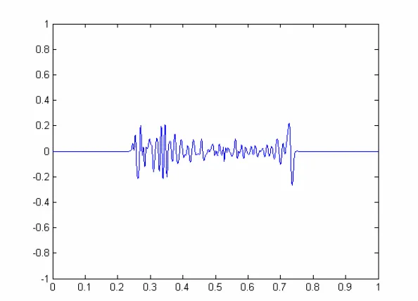
convolution of the pulse with the random medium and is shown in Fig.2.4.
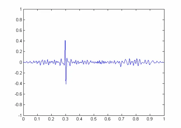
This signal (or a window of it) is then reversed in time, that is, the part of the signal
which came out of the medium first will re-enter the medium last, and vice versa. The
time reversed signal is then re-introduced into the same medium. The pulse that comes
out of the medium is again a convolution of the windowed complicated signal and the
random medium and will be similar in shape to the original pulse with a low amplitude
coda that can be seen in Fig.2.5.
2.3 TRAIN OF PULSES
We can also implement this method for a train of pulses. Here, instead of a single pulse,
we use a train of pulses, as shown in Fig.2.6. Compared to one pulse, a train of pulses can
carry considerably more information, and hence we can use the technique efficiently for
secure communication. Here the sequence is {1,0,1,0,0,1}.
Figure 2.6 Train of Gaussian pulses {1,0,1,0,0,1}
The pulse which goes first into the medium will come out last from the medium after
time reversal. The scales should always be kept in mind (ε2<<ε<<1 where ε is the
standard deviation of the original pulse and ε2 is the correlation length of the medium).
This train of pulses interacts with the random medium as shown in the Fig.2.2 and gives
Figure 2.7 Reflected signal when the Gaussian pulses interacts with the medium
This signal is then time reversed and is then sent back into the same medium which gives
us the pulses in the same sequence as we originally sent them into the medium (Fig.2.8).
A threshold level can be prescribed to detect the refocused pulse. This threshold can vary
depending on the application and amplitude of the original pulse. Here we can see the
sequence generated after time reversal to be {1,0,0,1,0,1} which is exactly the reverse of
Figure 2.8 Refocused train of pulses
The method is implemented using the C language on an 896 MHz Intel
Celeron-processor IBM ThinkPad. The time taken for computing the time-reversal wave for one
realization using 100 layers (N = 100) in this method is approximately 4 min 32 sec =
3. FINITE DIFFERENCE TIME DOMAIN (FDTD) METHOD
3.1 INTRODUCTION
Let h and k be positive numbers. We can define a grid by grid points (tn, xm) = (nk,mh)
for arbitrary positive integers n and m. For a function v defined on the grid we write vnm
for the value of v at the grid point (tn, xm). The set of points (tn,xm) for a fixed value of n
is called grid level n.
The basic idea of finite difference schemes is to replace derivatives by finite difference
approximations. For example:
ju/jt (nk,mh) = (u((n+1)k,mh)-u(nk,mh)))/k
= (u((n+1)k,mh)-u((n-1)k,mh))/(2k)
There are various finite difference schemes for the 1-D wave equation and several are
shown below:
(Vmn+1 – Vmn )/k + a . (Vm+1n – Vmn)/h = 0 (3.1)
(Vmn+1 – Vmn )/k + a . (Vmn – Vm-1n)/h = 0 (3.2)
(Vmn+1 – Vmn )/k + a . (Vm+1n – Vm-1n)/(2h) = 0 (3.3)
(Vmn+1 – Vmn-1 )/(2k) + a . (Vm+1n – Vm-1n)/(2h) = 0 (3.4)
(Vmn+1 – ½(Vm+1n + Vm-1n))/k + a . (Vm+1n – Vm-1n)/(2h) = 0 (3.5)
where Eq(3.1) – forward-time forward-space (2,2) scheme.
Eq(3.3) – forward-time central-space (2,2) scheme.
Eq(3.4) – Leapfrog (2,2) scheme.
Eq(3.5) – Lax-Friedrichs (2,2) scheme.
3.2 FORMULATION OF EQUATIONS:
We start with the 1-D wave equation:
j2u/jt2 (x,t) – α2j2u/jx2 (x,t) = 0, 0 < x < 1 and t > 0
subject to the following boundary and initial conditions -
u (0,t) = u (l,t) = 0, t > 0
u (x,0) = f (x), 0<=x<=l
ju/jt (x,0) = g(x), 0<=x<=l, where α= velocity of propagation.
To set up a finite difference method, select an integer m > 0 and time – step size k > 0.
With h=l/m, the mesh points (xi,tj) are defined as:
xi = ih for i = 0,1,2………m
tj = jk for j = 0,1,2,………N
At any interior mesh point (xi,tj), the wave equation becomes,
j2u/jt2 (xi,tj) – αi2j2u/jx2 (xi,tj) = 0 (3.6) The Finite difference method is obtained using the center – difference equation quotient
for the second partial derivatives given by:
where tj-1 < µj < tj+1
j2u/jx2 (xi,tj) = [u (xi+1,tj) – 2u (xi,tj) + u (xi-1,tj)]/h2 - h2/12 . j4u/jx4 (ξi,tj) where xj-1 < ξi < xj+1
Substituting these in Eq.(3.6) ,
[u (xi,tj+1) – 2u (xi,tj) + u (xi,tj-1)]/k2 - αi 2 . [u (xi+1,tj) – 2u (xi,tj) + u (xi-1,tj)]/h2
= 1/12 (k2 . j4u/jt4 (xi,µj) - α2h2 . j4u/jx4 (ξi,tj))
Neglecting the truncation error,
τi,j = 1/12 (k2 . j4u/jt4 (xi,µj) - αi 2h2 . j4u/jx4 (ξi,tj))
We have [ Wij+1 – 2Wij + Wij-1 ]/k2 - αi 2 [ Wi+1j -2Wij + Wi-1j ]/h2 = 0
We let λi = αi k/h and hence can write the difference equation as follows :
Wij+1 – 2Wij + Wij-1 – λi 2Wi+1j + 2 λi 2Wij - λi 2 Wi-1j = 0
and then solve for Wij+1 , the most advanced time-step approximation, to obtain
Wij+1 = 2(1 - λi 2)Wij + λi 2 (Wi+1j + Wi-1j )- Wij-1 (3.7)
This equation holds for each of i = 1,2…(m-1) and j = 1,2…(N-1)
The velocities of propagation αi for each layer ‘i’ can be seen in Fig 3.1. This method
gets slower as we increase the number of points per layer. The least number of points we
wave equation using the (2,2) explicit scheme. So, in order to demonstrate time-reversal,
we use 2 points per layer.
As the discretization of the wave equation is second order accurate in time and second
order accurate in space, this scheme is called (2,2) explicit scheme. It is called ‘explicit’
because the current value of the solution of the wave equation can be explicitly obtained
from its previous values.
3.3 BOUNDARY CONDITIONS AND HIGHER ORDER ACCURATE SCHEMES
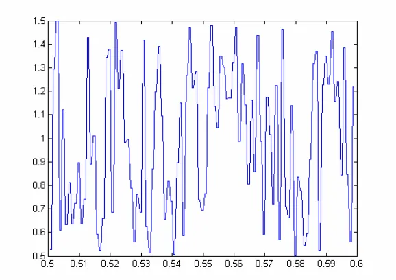
Our domain for demonstrating the time reversal is the interval [0,1]. The scatterer is
located between 0.5 and 0.6 in this space with the Gaussian pulse initially to the left of
the scatterer. We assume that the signal does not reach the boundaries of the domain.
Thus, in this case, the wave propagation can be subject to the following boundary
conditions:
W0j = Wmj = 0 j = 1,2……N
Equation (3.7) is the (2,2) explicit scheme and requires a stencil of 3 mesh points, one on
each side of the mesh point on which the calculation is to be done. We can also have
higher order accurate schemes for the second order equations. One such scheme is the
second order in time and fourth order in space ((2,4) scheme). This can be written as
follows:
We let λi = αi k/h and hence can write the difference equation as follows :
Wij+1 = 2Wij - Wij-1 + (λi 2/12)( - Wi+2j + 16Wi+1j -30Wij + 16Wi-1j - Wi-2j ) (3.8)
This equation requires a stencil of 5 mesh points, two on each side of the mesh point on
which the calculation is to be done. This method gives us more accurate results compared
to the (2,2) scheme but increases the computational complexity.
3.4 ALGORITHM
The algorithm used for implementing time reversal using the FDTD method employs the
(2,4) scheme discussed above. As this scheme requires 2 mesh points on each side of the
mesh point on which the calculation is being done, the second and the second last mesh
point uses the (2,2) scheme to evaluate values at those mesh points.
We approximate Wij to u (xi, tj) for each i = 0,1,2…….m & j = 0,1,2……..N and
thereafter proceed to the following steps of the algorithm:
Step 1: Set h = l/m
k = T/N
λ= kα/h
where l = Endpoint, T = Maximum time , α = Constant and m, N = Integers
Step 2: For j = 1,2,……….N, W0j = Wmj = 0
Step 3: Set W00 = f (0)
Step 4: For i = 1,2,……m-1 (Initialize for t=0 & t=k)
Set Wi0 = f (ih)
Wi1 = (1 – λ2) f (ih) + λ2/12 [ f ((i+1)h) + f ((i-1)h) ] + k g (ih)
Step 5: For j = 1,2……..N-1
For i = 1,2,………m-1
if i = 1 or i = m-1
Set Wij+1 = 2(1 - λ2)Wij + λ2 (Wi+1j + Wi-1j )- Wij-1
else
Set Wij+1 = 2Wij - Wij-1 + (λ2/12)( - Wi+2j + 16Wi+1j -30Wij
+ 16Wi-1j - Wi-2j )
Step 6: For j = 0,1,2 …….N
Set t = jk
For i = 0,1,2…….m
Set x = ih
OUTPUT = (x, t, Wij)
Step 7: END
3.5 RESULTS
The implementation of time reversal in 1-D is done in accordance with the algorithm in
the previous section. We create a random complex medium using the random number
generator to determine the velocities in various layers of the medium. All the
computations are done and results presented using MATLAB 5 on an 896 MHz Intel
Celeron-processor IBM ThinkPad. The medium can be seen in Fig 3.1.
Figure 3.1 Distribution of the velocity of propagation of the random medium
For implementing time reversal using this method, we can start with any pulse. Here the
pulse used is a Gaussian pulse defined by the equation:
Figure 3.2 Initial Gaussian pulse
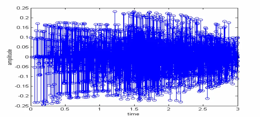
This pulse, when propagated through the random complex media, gives rise to a reflected
signal and a transmitted ( refracted ) signal. This can be seen in the Fig 3.3.
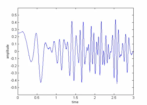
To demonstrate time reversal of the reflected signal, the reflected wave is then taken and
sent through the same complex random medium after time reversal i.e. the part of the
signal that comes out first will go in last into the medium (LIFO). This gives rise to pulse
refocusing and we can see a pulse which is of the same shape as the original pulse, and
reduced amplitude because we are storing only the reflected wave and also due to some
loss of energy due to propagation. The refocused pulse can be seen in the Fig 3.4.
Figure 3.4 Refocused pulse
Fig. 3.5 is the magnified view of the refocused pulse. This can be used to study
characteristics of the refocused pulse and the amplitude of the refocused pulse can be
Figure 3.5 Magnified view of the refocused pulse
3.6 DIFFERENT REALIZATIONS USING VARIOUS RANDOM MEDIA
Fig 3.6 shows the refocused pulse for 10 different realizations using different complex
media each having N=100 layers and velocities of propagation distributed uniformly
between 0.5 and 1.5. It can be seen clearly that for each of the realizations, the position
and the amplitude of the pulse is independent of the way the velocities in the complex
media are assigned. Only the low-amplitude coda around the pulse is different for
different random complex medias. Hence we can say that the pulse refocuses in a manner
that is self-averaging with respect to random realizations of wave speed in the component
layers of the random complex media.
3.7 NUMERICAL CONVERGENCE AND TIME CONSIDERATIONS
The most basic property that a scheme must have in order to be useful is that its solutions
approximate the solution of the corresponding partial differential equation and that the
approximation improves as the grid spacing h and k, tend to zero. We call such a scheme
a convergent scheme. The grid spacing will tend to zero as we increase the number of
points per layer for each of the layers. In our (2,4) explicit scheme, as we increase the
number of points per layer, the refocused pulse amplitude converges to some limiting
amplitude and use this as a measure of the extent to which the method has numerically
converged. The execution time to achieve the refocused pulse for one realization having
5 using 896 MHz Intel Celeron-processor IBM ThinkPad. This makes it clear that the
4. BOUNDARY INTEGRAL METHOD
4.1 INTRODUCTION
The boundary integral scheme is formulated in the frequency domain. This method is
based on Green’s functions and is very efficient in dealing with problems in 1-D
involving interface conditions. We start with the definition of the Fourier Transform
followed by an explanation of the method which involves the Hemholtz equation. We
define the Fourier Transform as follows:
∫
∞
∞ −
≡ e u x t dt uˆ( ) i t ( , )
: Transform
Fourier ω ω
Using this definition, we write the wave equation:
j2u/jt2 (x,t) – α2j2u/jx2 (x,t) = 0
in the frequency domain by taking Fourier Transform of each of its terms. The
representation in the frequency domain reduces to Helmholtz equation:
) 2 . 4 ( ) / ( ) , ( ) , ( , 0 ) , ( ˆ ) , ( ˆ ) 1 . 4 ( ) / ( , 0 ) , ( ˆ ) , ( ˆ ) < < : Equation Helmholtz 0 2 2 2 2 c k a a x x u k x u c k x x u k x u N x j j j x ω ω ω ∂ ω ω ω ∂ ω = ∞ ∪ −∞ ∈ = + = Ω ∈ = + ∞ ∞
where layer ‘j’ can be represented by Ωj=(aj,aj+1) and aj and aj+1 represents the two
Now we introduce Green’s function for each domain that satisfy: (4.4) ) , ( ) , ( , , ) ( ) , , ( ˆ ) , , ( ˆ (4.3) , , ) ( ) , , ( ˆ ) , , ( ˆ ) < < (-: subdomain each for Functions s Green' 0 2 2 2 2 ∞ ∪ −∞ ∈ − = + Ω ∈ − = + ∞ ∞ N x j j j j x a a y x y x y x H k y x H y x y x y x H k y x H δ ω ω ∂ δ ω ω ∂ ω
where δ (x) is the Dirac delta function. For an incident wave that propagates from left to
right, the Green’s function that satisfy the above two equations are respectively:
) , ( ) , ( , , 2 ) , , ( ˆ , , 2 ) , , ( ˆ 0 | | | | ∞ ∪ −∞ ∈ = Ω ∈ = − − N y x ik j j y x ik j a a y x ik e y x H y x ik e y x H j ω ω
4.2 ASSEMBLY OF THE SYSTEM OF EQUATIONS
We multiply Equation (4.3) by uˆ(x)and (4.2) by Hˆ j(x,y) and then subtract one
equation from the other. Integrating the above expression along the region between the
two interfaces would give us the expression at any point.
∫
∫
∫
+ − = + − + ∈ + 1 1 1 ) ( ˆ ) , ( ˆ ) ( ˆ ) , ( ˆ ) ( ) ( ˆ : ) , ( For 2 2 1 j j j j j j a a x j a a j x a a j j dx x u y x H dx x u y x H dx y x x u a a y ∂ ∂ δ) ( ˆ ) , ( ˆ ) ( ˆ ) , ( ˆ ) ( ˆ ) , ( ˆ ) ( ˆ ) , ( ˆ ) ( ˆ 1 1 1 1 j x j j j x j j j j j x j j j x a u y a H a u y a H a u y a H a u y a H y u ∂ ∂ ∂ ∂ + − − = + + + +
We obtain a closed system of linear algebraic equations for the unknown quantities on the
interfaces by taking the limit as the interior point y approaches the end points of each
interval (aj,aj+1). ) ( ˆ ) , ( ˆ ) ( ˆ ) , ( ˆ ) ( ˆ ) , ( ˆ ) ( ˆ ) , ( ˆ ) ( ˆ ) ( ˆ ) , ( ˆ ) ( ˆ ) , ( ˆ ) ( ˆ ) , ( ˆ ) ( ˆ ) , ( ˆ ) ( ˆ 1 1 1 1 1 1 1 1 1 1 1 1 1 1 j x j j j j x j j j j j j j x j j j j x j j j x j j j j x j j j j j j j x j j j j x j j a u a a H a u a a H a u a a H a u a a H a u a y a u a a H a u a a H a u a a H a u a a H a u a y ∂ ∂ ∂ ∂ ∂ ∂ ∂ ∂ − + + − + + − + + − + + + − + + + + + + + + + + + − − = ⇒ → + − − = ⇒ →
These two equations comprise 2N equations in the 2N+2 unknowns consisting of the
values of uˆ and ∂xuˆ on the interfaces located at y=a0……..y=aN known as the Layer
Two additional equations are obtained by performing a similar limit analysis on the
intervals (-∞,a0) and (aN, ∞) and hence complete the formulation of a closed system of
linear algebraic equations for the interface unknowns.
0 ) ( ˆ 2 1 ) ( ˆ 2 1 : , Let . ) , ( : scatterer of end Right ) ( ˆ 2 1 ) ( ˆ 2 1 : , Let ). , ( : scatterer of end Left 0 0 0 0 0 = − → ∞ → ∈ = + → ∞ → − ∈ + − N x N N N ika x a u ik a u a y L L a y e a u ik a u a y L a L y ∂ ∂
Now we can use this method for a specific incident pulse. We consider a Gaussian pulse
centered at y=y0 and having velocity c with variance δ.
2 1 ) ( : pulse
Incident ( ) /(2 )
0 2 2 0 δ δ π ct y y e ct y y
f − − = − − −
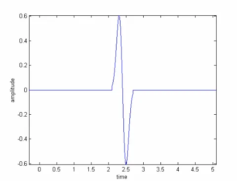
The incident pulse used for the simulation is the first derivative of the Gaussian pulse.
The following equation gives the formula for the refocused pulse after time reversal for a
incident pulse (derivative of Gaussian) centered at y0 with variance = δ.
4.3 PULSE REFOCUSING AND RANDOM REALIZATIONS
To get the pulse refocusing via time-reversal in 1-D using this method, we can start with
a Gaussian derivative pulse defined by the equation:
f(t)= - (t/√ε)*exp(-t2/2*ε)
and shown in Fig. 3.2. We then formulate the set of equations discussed in the previous
section to get the refocusing of the pulse.
Here we set the number of layers, N=100, the length of sampling interval t0 = 3.0 and
variance of the pulse δ = 0.01. The refocused pulse is shown in the Fig 4.1 below.
Implementing Time reversal using multiple realizations of the medium and plotting
results on the same axes helps us conclude that the shape of the refocused pulse is
independent of the realization of the medium.
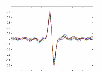
We can demonstrate this self-averaging property by taking 10 different realizations for
N=100 and velocities of propagation generated using a random number generator. All the
computations are done and results presented using MATLAB 5 on an 896 MHz Intel
Celeron-processor IBM ThinkPad
Figure 4.2 10 Random realizations of the refocused pulse
4.4 EFFECT OF INCREASING THE NUMBER OF LAYERS:
Here we illustrate the refocusing of the time-reversed pulse as the number of layers N in
the scatterer is increased. For each N, we computed the time-reversed pulse for 10
different realizations of the scatterer. As more layers are added to the scatterer, the
In this regime, the self-averaging property of the refocused pulse becomes more
pronounced which can be seen by comparing the figures below. The characteristic
wavelength of the refocused pulse is on the same scale as the original incident pulse. As
N increases we can have a direct comparison of the numerical simulations to the
theoretical results (N→∞).
Figure 4.3 10 Random realizations of the refocused pulse (N=5)
Figure 4.4 10 Random realizations of the refocused pulse (N=10)
Figure 4.5 10 Random realizations of the refocused pulse (N=20)
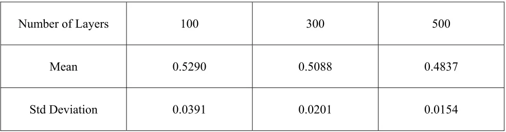
Table 1 below shows the comparison of the standard deviations of the amplitudes of the
refocused pulse for 25 different realizations with number of layers N = 100, 300 and 500.
Table 1: Study of effect of increasing the number of layers on the pulse amplitude for 25
different realizations
Number of Layers 100 300 500
Mean 0.5290 0.5088 0.4837
Std Deviation 0.0391 0.0201 0.0154
We observe that as we increase the number of layers N, the variation (standard deviation)
in the amplitude of the refocused pulse reduces significantly and tends to some limiting
theoretical value.
Figure 4.7 10 Random realizations of the refocused pulse (N=100)
4.5 VERIFICATION OF THE THEORETICAL FORMULA:
Time reversal in 1-D has been implemented using 3 different methods and it is seen that
the self-averaging property can be demonstrated using each of those methods. Here will
be compare the numerical results achieved using the Boundary Integral Method to the
theoretical formula for the time reversed pulse. We start the analysis with our incident
pulse given by:
f(t) = d/dt(exp(-t2/2))
= t . exp(-t2/2)
If our velocities of propagation are defined for different layers as:
1/c2 = 1+µ(x) where µ(x) = U (-0.8 0.8)
Then we calculate ‘α’ called the integrated correlation as follows:
375 / 128 ] 3 / 3 [ )] ( ) 0 ( [ 8 . 0 8 . 0 8 . 0 8 . 0 2 0 = = = = − − ∞
∫
∫
x dx x dx xE µ µ
α
Once you have the integrated correlation, the refocused pulse is given by:
where Ht0’(t) = some kernel function
=F-1[Λ(w, .) * Gt0’(- .)] (0)
with Λ(w, .) = αw2/(1+w2αt)2 and Gt0’(- .) = cutoff function between 0 to t0’.
Using these two expressions we calculate the kernel function.
) ' 1 /( ' ) 1 /( ) , ( ) ( ) , ( ) 0 )]( ( * ) , ( [ 0 2 0 2 ' 0 2 2 2 ' 0 0 ' . ' 0 . 0 0 t w t w d w w d w d G w G w t t to t α α τ ατ α τ τ τ τ τ + = + = Λ = Λ = − Λ
∫
∫
∫
∞Hence, fTR(t) = (f * Ht0’) (t)
= F-1 [f(w) . Ht0’(w)]
dw t w t w w f
e iwt . ( ). '/(1 ') 2
/
1 2 0
0
2 α
α +
Π
=
∫
−where f(w) = F [ f(t) ] = -iw exp(-w2/2)
Therefore f t e iwt iw e w w t w t dw
TR( ) 1/2 .( . ). '/(1 0')
2 0 2 2 / 2 α α + − Π =
∫
− −This is the final pulse which we get after time reversal. This is compared with the
numerical results for varying number of layers and results show that for sufficiently large
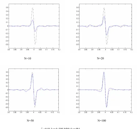
In the Fig 4.9 the dotted line indicates the theoretical time reversed pulse and the solid
lines indicate numerical results for the mean curve over 10 different realizations with
varying number of layers. It can be seen clearly that as we increase the number of layers
N, the numerical result approaches the theoretical formula.
Figure 4.9 Verification of theoretical formula for different number of layers
N=10 N=20
N=50 N=100
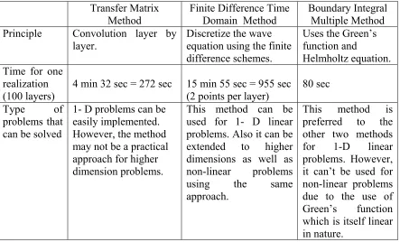
Table 2 gives a very clear picture that while addressing a problem in 1-D which is linear
in nature, the Boundary Integral Method is preferable to the other two methods. However,
if we address problems in 2-D and 3-D or problems having a non-linear property then the
FDTD method may be necessary.
Table 2: Comparative Study of the three methods in terms of speed and accuracy.
Transfer Matrix
Method
Finite Difference Time Domain Method
Boundary Integral Multiple Method Principle Convolution layer by
layer.
Discretize the wave equation using the finite difference schemes.
Uses the Green’s function and
Helmholtz equation. Time for one
realization
(100 layers) 4 min 32 sec = 272 sec 15 min 55 sec = 955 sec (2 points per layer) 80 sec Type of
problems that can be solved
1- D problems can be easily implemented. However, the method may not be a practical approach for higher dimension problems.
This method can be used for 1- D linear problems. Also it can be extended to higher dimensions as well as non-linear problems using the same approach.
5. DETECTION OF A BURIED CAVITY VIA TIME-REVERSAL
5.1 HYPOTHESIS
After having implemented time-reversal in 1-D successfully using the Boundary Integral
Method, its potential for being used in various applications such as detection of a
cavity/object buried in a random layered scatterer is now analyzed. We hypothesize that
time-reversal detection can be evaluated by comparing the amplitude of the time-reversed
pulse for a realization of the layered medium to the amplitude of the time-reversed pulse
for the same realization of the layered medium with a hollow cavity. It will be seen that
the amplitude of the time-reversed pulse can be used as a measure for detection of a
cavity buried in a random layered scatterer. Statistics of the time reversed pulse
amplitude for several cases is also shown which helps in making some useful deductions
about the presence and size of the target to be detected.
5.2 EXPERIMENTS
Numerical simulations were conducted on the scales N = 100, δ = 0.01 with the wave
numerical convergence of the refocused pulse for a single realization of the scatterer was
roughly 80 seconds. While the chosen scales are relatively coarse, our simulations
illustrate the potential for using the self-averaging property of the time-reversed pulse in
detection of a buried cavity. The cavity is introduced by removing L/2 layers on either
side of a specified location y = yc within the scatterer. To illustrate the effect of a cavity
on the amplitude of the refocused pulse, a sample realization in the case where L = 50, yc
= 0.5, t* = 2.0, t0 = 3.0 is shown in Fig 5.1. We observe that the pulse amplitude drops in
the presence of a buried cavity (Figure 5.1). This drop in the amplitude of the refocused
pulse suggests presence of a buried object/cavity in the medium.
Figure 5.1 Comparison of pulse amplitude with and without cavity
The amplitudes of the pulse with and without cavity are compared for 50 different
realizations (Figure 5.2). We can see that the amplitude of the pulse without cavity almost
Figure 5.2 Comparison of pulse amplitudes with and without cavity for 50 realizations
We consider a detailed analysis for using the refocused pulse as a measure to detect
buried targets. We observe that the amplitude of the refocused pulse is a good indicator
and shows a promise for detecting buried objects/cavity.
As a specific detection measure of the time-reversed pulse, we choose the signed
percentage difference between the two pulse amplitudes:
(i.e. [(no cavity)-(cavity)]/(no cavity))
For yc = 0.5, t* = 2.0 and t0 = 3.0, this measure is plotted for 50 realizations in the cases
Figure 5.3 % difference of the amplitudes with and without cavity (L=50) for 50
realizations
The values of the signed percentage difference can help us deduce the size of the object.
To study this, we can compare the result in Fig 5.3 with results of various other values of
L. The Fig 5.4 below shows the signed percentage difference for L=20, 10 and 4.
We can deduce the size of the buried object/cavity using the results in the figure above.
The size of the object/cavity appears to increase with the value of the percentage
5.3 STATISTICAL ANALYSIS OF TIME REVERSED PULSE AMPLITUDE:
Statistics of this detection measure indicate the mean percentage difference increase with
L. On the scales considered, these values indicate that this detection measure is a good
indicator of the presence of a relatively large buried cavity. The values of the
time-reversed pulse amplitude for several cases are shown in Table 3.
% difference for L=20 % difference for L=10
% difference for L=4
Table 3: Statistics of time-reversed pulse amplitude for different size of object/cavity for number of layers N=100. Mean values are reported with standard deviations in parentheses.
Case t0 L yc Amplitude
(no cavity) Amplitude (cavity) Signed % difference 1 3.0 50 0.5 0.479 (0.055) 0.320 (0.050) 33.37% (5.75%)
2 3.0 20 0.5 0.479 (0.055) 0.432 (0.049) 9.84% (5.55%)
3 3.0 10 0.5 0.479 (0.055) 0.455 (0.051) 5.31% (4.72%)
4 3.0 4 0.5 0.479 (0.055) 0.465 (0.053) 3.11% (4.82%)
The values of the signed percentage difference show promise for using time-reversal to
detect the size of a buried cavity. We can see that the percentage difference decreases as
we reduce the value of L. Hence, the percentage difference in the amplitudes of the
refocused pulse with and without the cavity/object is a good indicator of the size of the
object/cavity.
Table 4 indicates the extent to which the detection measure can indicate the depth of a
buried cavity when L=20 and yc = 0.67. By increasing t0 when t* = 2.0, we simulated the
effects of gradually increasing the duration of the recording window for the reflected
Table 4: Statistics of time-reversed pulse amplitude to analyze the extent to which the detection measure can indicate the depth of buried cavity for N=100. Mean values are reported with standard deviations in parentheses.
Case t0 L yc Amplitude
(no cavity) Amplitude (cavity) Signed % difference 1 0.8 20 0.67 0.260 (0.066) 0.258 (0.062) 0.11% (1.70%)
2 1.0 20 0.67 0.299 (0.070) 0.300 (0.068) 0.11% (0.92%)
3 1.2 20 0.67 0.330 (0.075) 0.327 (0.072) 0.78% (2.34%)
4 1.5 20 0.67 0.376 (0.066) 0.345 (0.078) 8.99% (8.24%)
5 2.0 20 0.67 0.435 (0.055) 0.390 (0.065) 10.30% (8.00%)
6 3.0 20 0.67 0.480 (0.060) 0.425 (0.065) 10.52% (7.99%)
For smaller values of t0 (Cases 1-3), we observe that the detection measure does not
indicate any significant drop in pulse amplitude in the presence of the buried cavity. As t0
is increased, the percentage difference increased when the time-reversal window
incorporates portions of the reflected signal that correlates to the depth in the scatterer at
which the cavity is buried (Cases 4-6). More extensive studies are required to determine
specific relations between the critical value of the recording duration t0 for the reflected
For the layer resolution considered in this study (N = 100), the amplitude of the
time-reversed pulse is a good indicator of the presence or absence of a relatively large
buried cavity (of length L). The time-reversed pulse also shows promise as an indicator
of cavity size and depth within the scatterer, although more extensive parametric studies
6. CONCLUSIONS AND FUTURE WORK
Time reversal of waves propagating in random media was successfully implemented
using the three different methods. In particular, the results of 1-D time reversal using the
Boundary Integral Method was shown to be more precise and faster compared to Finite
Difference Time Domain Method and the Transfer Matrix Method. Furthermore, it is also
shown that Time reversal mirrors of waves propagating in random media shows promise
as a potential candidate for underground or buried object / cavity detection using the
amplitude of the refocused pulse as an indicator. This principle can be extended for
mine-detection purpose to detect the presence of all individual mines.
Here time reversal is implemented in one spatial domain. This method can be extended to
2-D and 3-D cases and hence become useful for more practical applications. Future work
would also include conducting a more extensive set of simulations on finer scales. More
detailed simulations of the detection inverse problem can be studied on finer scales by
increasing N by at least one order of magnitude. Better extensive studies are required to
determine specific relations between the critical value of the recording duration t0 for the
reflected signal and the depth yc of the buried cavity. Scaling parameters including the
characteristic pulse wavelength δ, sampling duration t0 and sampling time t* can be
optimized to enhance the self-averaging properties of time-reversal in the context of
Time reversal mirrors are not only devoted to applied physics. They can also be used in
fundamental physics to solve problems in the field of wave propagation. Inverse
problems can be solved by the use of a time reversal mirrors which can also be used to
study multiple-scattering processes in heterogeneous media and to give some new
approaches to the problem of wave localization.
Time reversal techniques may also be extended to types of waves other than acoustic
waves. Some researchers in the radar community are exploring their possible application
to pulsed radar, using electromagnetic waves in the microwave range. Another type of
wave occurs in quantum mechanics: the quantum wavefunctions that describe all matter.
Indeed, a type of retroreflection can occur when an electron wavefunction hits the
boundary between a normal conductor and a superconductor. One can only speculate on
what kinds of tricks would be possible if time reversal were applied to the waves of
quantum mechanics.
Plenty of exploration can be done in the field of medical applications using time reversal.
Abdominal and cardiac applications are limited by the motions of breathing and
heartbeats which can use the time reversal technique. Also another challenge is the brain
hyperthermia in which we need to focus through the skull, which severely refracts and
scatters the ultrasonic beam. The porosity of the skull produces a strong dissipation –
absorbing energy from the wave – and thus breaks the time-reversal symmetry of the
wave equation. A new focusing technique can be developed using time reversal that adds
7. REFERENCES
[1] T. Yu and L. Carin, "Extended-Born method for the modeling of buried voids", IEEE
Trans. Geoscience and Remote Sensing, vol. 38, pp. 1320-1327, May 2000
[2] Asch M, Kohler W, Papanicolaou G, Postel M and White B 1991 Frequency content
of randomly scattered signals SIAM Review 33 pp 519-625
[3] Asch M, Papanicolaou G, Postel M, Sheng P, and White B 1990 Frequency content of
randomly scattered signals, Part I, Wave Motion 12 pp 429-450
[4] M. Porter, P. Roux, H. Song, and W.A. Kuperman, "Tumor treatment by
time-reversal acoustics," IEEE Proc. ICASSP-99, IV-2107, Phoenix, Arizona, 1999.
[5] Bal G and Ryzhik L 2002 (preprint).
[6] J.P. Fouque and A. Nachbin: Time-reversed refocusing of surface water waves
Submitted 2002.
[7] Blomgren P, Papanicolaou G and Zhao H 2002 Super-resolution in time-reversal
acoustics JASA 111 pp 230-248
[8] G.F. Edelmann, W.S. Hodgkiss, S. Kim, W.A. Kuperman, H.C. Song, and T. Akal,
"Underwater acoustic communication using time reversal," Oceans 2001, Hawaii, 2001.
[9] Borcea L, Tsogka C, Papanicolaou G and Berryman J 2002 Imaging and time-reversal
in random media Inverse Problems 18 pp 1247-79
[10] J.P. Fouque, J. Garnier and A. Nachbin: Time reversal for dispersive waves in
[11] S. Kim, W.A. Kuperman, W.S. Hodgkiss, H.C. Song, G.F. Edelmann, T. Akal, R.P.
Millane, D. Di Iorio, "A method of robust time reversal focusing in a fluctuating ocean,"
Oceans 2001, Hawaii, 2001.
[12] Clouet J F and Fouque J P 1997 A time-reversal method for an acoustical pulse
propagating in randomly layered media Wave Motion 25 pp 361-8
[13] Fink M 1993 Time reversal mirrors J. Phys. D: Appl. Phys. 26 pp 1333-1350
[14] Fink M 1999 Time-reversed acoustics Scientific American, November 1999,
pp.67-93
[15] H.C. Song, W.A. Kuperman, W.S. Hodgkiss, T. Akal, S. Kim, and G. Edelmann,
"Recent results from ocean acoustic time reversal experiments," 6th European
Conference on Underwater Acoustics, Gdanski, Poland, 2002.
[16] Fouque J P and Sølna K 2002 Time-reversal aperture enhancement, submitted
[17] Haider M A, Shipman S P and Venakides S 2002 Boundary-integral calculations of
two-dimensional electromagnetic scattering in infinite photonic crystal slabs: channel
defects and resonances SIAM J Appl. Math 62, pp 2129-48
[18] Papanicolaou G, Postel M, Sheng P and White B 1990 Frequency content of
randomly scattered signals, Part II, Wave Motion 12 pp 527-49
[19] W.A. Kuperman, H.C. Song, and P. Roux, "Focal translation by frequency shift with
a time-reversal mirror," First International Symposium on Physics in Signal and Image
Processing (PSIP), Paris, France, 1999.
[20] Rokhlin V 1990 Rapid solution of integral equations of scattering theory in two
[21] L.Carin, R. Kapoor, C.E. Baum, "Polarimetric SAR imaging of buried landmines,"
IEEE Trans. Geoscience and Remote Sensing, vol. 36, pp. 1985-1988, Nov. 1998.
[22] D. Wong and L. Carin, "Analysis and processing of ultra-wideband SAR imagery
for buried landmine detection”, IEEE Trans. Antennas Propagation, vol. 46, pp.
1747-1748, Nov. 1998.
[23] L. Carin, N. Geng, M. McClure, J. Sichina, and L. Nguyen, "Ultra-wideband
synthetic aperture radar for mine field detection”, IEEE Antennas and Propagation
Magazine (invited), vol. 41, pp. 18-33, Feb. 1999.
[24] L. Collins, P. Yao, and L. Carin, "A Bayesian theoretic algorithm for detection of
land mines", IEEE Trans. Geoscience and Remote Sensing, vol. 37, pp. 811-819, Mar.
1999.
[25] NUMERICAL ANALYSIS ( 4th Edition ) by Richard Burden & J. Douglas Faires.
[26] FINITE DIFFERENCE SCHEMES & PARTIAL DIFFERENTIAL EQUATIONS
by John C. Strikwerda.
[27] http://www.gis.wau.nl/sar/sig/sar_intr.htm