Mobility Profiling for Mobile Trajectory Based Services.

ABSTRACT

KHOKHAR, SARFRAZ.Mobility Profiling for Mobile Trajectory Based Services. (Under the direction of Prof. Arne A. Nilsson).

Mobility Profiling for Mobile Trajectory Based Services

by

Sarfraz Khokhar

A dissertation submitted to the Graduate Faculty of

North Carolina State University

in partial fulfillment of the

requirements for the Degree of

Doctor of Philosophy

Computer Engineering

Raleigh, North Carolina

2008

APPROVED BY:

______________________________ ___________________________

Dr. Arne A. Nilsson Dr. Harry G. Perros

(Chair of Advisory Committee

)

ii

DEDICATION

iii

BIOGRAPHY

Sarfraz Khokhar received his BSc in Math and Physics from Punjab University Lahore, Pakistan and MSc in Electronics from Quaid-i-Azam, Islamabad, where he was valedictorian and received a gold medal from the president of the country and was offered a faculty position at the same university. In June, 1989, he won a CERN fellowship in an international competition. He worked on the famous LEP Collider, where he got a chance to work directly with famous scientists and Nobel Laureates. Along with high-energy physics, he worked on high speed networking projects.

iv

ACKNOWLEDGMENTS

v

TABLE OF CONTENTS

List of Figures

………..………..

viii

List of Tables ……….…..…………....……

xi

Chapter 1

Introduction

...

1

1.1 Challenges in Mobility Profiling ... 3

1.2 Geo-spatial Technology in LBS ... 5

1.3 Location Comparison with Map ... 6

1.4 Proposed Mobility Profiling... 7

1.5 Contributions and Organization of the Thesis ... 8

1.5.1 Introduction of MTBS and Their Provisioning Architecture ... 8

1.5.2 Road Network and Mobile Trajectory Framework ... 8

1.5.3 MAP Digitizing Software Application ... 9

1.5.4 Mobility Profiling Algorithm and Simulation ... 9

1.5.5 Organization of the Thesis ... 10

Chapter 2

Location Estimation Technologies and Location Based Services

...

11

2.1 LBS System Architecture ... 12

2.2 Location Estimation Technologies ... 13

2.2.1 Time-Based Methods ... 15

2.2.1.1 Time of Arrival ... 16

2.2.1.2 Time Advance ... 19

2.2.1.3 Time Difference of Arrival and Observed Time Difference ... 21

2.2.2 Angle of Arrival... 26

2.2.2.1 Conventional Methods ... 28

2.2.2.2 Multipath Propagation Modeling in AOA ... 29

2.2.3 Signal Attenuation ... 31

2.2.4 Assisted-GPS ... 32

2.3 Location Information ... 35

2.4 Map-matching Survey ... 36

2.5 Location Based Services ... 39

2.5.1 Location Accuracy and LBS ... 41

2.5.2 Middleware System ... 43

2.5.3 Key Protocols in LBS ... 46

2.5.3.1 WAP ... 46

2.5.3.2 Mobile Location Protocols (MLP) ... 52

2.5.3.3 MLP Structure ... 53

Chapter 3

Mobile Trajectories- The Objective

...

56

3.1 Examples of MTBS ... 57

3.2 Issues to Overcome in Trajectory Estimation ... 58

3.2.1 Hearability of Remote BSes ... 58

vi

3.2.3 Non–Line of Sight (NLOS) Conditions ... 59

3.2.4 Geometric Dilution of Precision (GDOP) Caused by Suboptimal BSes Layout . …...60

3.3 Polling Frequency ... 62

3.4 Additional Benefits of Mobility profiling ... 66

3.4.1 Smooth Handoff ... 66

3.4.2 Optimized Cell Sectorization ... 66

3.4.3 Early Channel Allocation ... 67

3.4.4 Code and Frequency Reuse in Micro Cell ... 67

Chapter 4

Mobility Profiling

...

68

4.1 GIS ... 68

4.1.1 GIS Data Standards and Architecture ... 70

4.1.2 Digital Road Databases ... 71

4.1.3 Mobile GIS ... 73

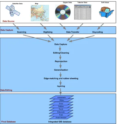
4.1.4 Creating A GIS Database ... 74

4.1.5 Manual Digitization ... 76

4.2 Map-matching ... 79

4.2.1 Geometric Point-to-Point Matching ... 80

4.2.2 Geometric Point-to-Curve Matching ... 81

4.2.3 Geometric Curve-to-Curve Matching ... 83

4.3 Geometric and Topological Information ... 84

4.4 Shape Matching ... 84

4.4.1 Shape Descriptors ... 85

4.4.2 Turning Function ... 86

4.5 Similarity Measures ... 86

4.5.1 A similarity Measure Based on the Turning Function ... 86

4.5.2 Hausdorff Distance ... 87

4.5.3 Fréchet Distance ... 88

4.5.4 Bounded Area ... 89

4.6 Mobility Profiling and MTBS Provisioning System Architecture ... 90

4.7 MobilityProfiling Theoretical Framework ... 91

4.7.1 Road Network Element ... 92

4.7.2 Road Network Representation ... 93

4.7.3 Metric Spaces Framework ... 94

4.7.4 Road Network in Topological Space... 98

4.7.5 Road Network’s Length Structure ... 103

4.7.6 Paths in a Road Network ... 104

4.7.7 Path Length on a Road Network ... 105

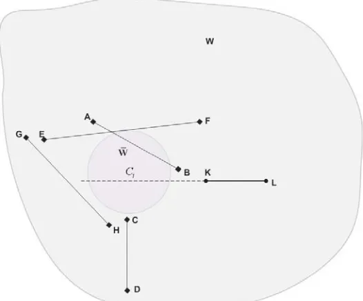
4.7.8 Closed Ball Embedded in Mobile User Space ... 108

4.7.8.1 Geodesic Candidacy ... 110

4.7.8.2 Estimated Location Correction within an Error Ball ... 113

4.7.8.3 Discrete Error Balls ... 121

4.7.8.4 Error Ball’s Directional Orientation ... 128

4.7.8.5 Direction Negativity ... 130

4.7.8.6 Path between the Corrected Points ... 131

4.8 MobilityProfiling Steps ... 132

vii

Chapter 5

Trajectory Estimation Simulation

...

137

5.1 Road Network MAP digitization ... 137

5.2 Location Estimation Simulation ... 144

5.3 Mobility Profiler ... 146

Chapter 6

Results and Conclusion

...

151

6.1 Trajectory Estimation ... 151

6.2 Trajectory Error Index ... 151

6.2.1 Linear Error ... 152

6.2.2 Areal Error ... 152

6.3 Trajectory Estimation Simulation Results ... 153

6.4 Simulation Conclusion ... 159

6.5 Comparison ... 160

Chapter 7

Future Research

...

172

7.1 Road Network Data Representation as Splines ... 172

7.2 Trajectory Legs Partitions ... 172

7.3 Travel Path Constraint ... 173

7.4 Location Error Modeling ... 173

7.5 Trajectory Estimation Algorithm Refinement ... 173

viii

LIST OF FIGURES

Figure 1.1: A conceptual comparison of LBS and MTBS

... 3

Figure 1.2: GIS high-level architecture

... 5

Figure 1.3: High level GIS layers representation

... 6

Figure 2.1: LBS communication model

... 11

Figure 2.2: End-to-End LBS system architecture

... 13

Figure 2.3: Location estimation with TOA

... 16

Figure 2.4: Location feasible area

... 18

Figure 2.5: TA compared with other legacy location techniques

... 20

Figure 2.6: Location estimation with TDOA

... 21

Figure 2.7: Generalized Cross-Correlation method

... 25

Figure 2.8: Location estimation with AoA

... 27

Figure 2.9: Delay-and-sum method

... 28

Figure 2.10: AoA scattering

... 30

Figure 2.11: MS lies on the circle where signal strength is the same

... 31

Figure 2.12: Membership function

... 32

Figure 2.13: A-GPS for location estimation

... 34

Figure 2.14: A-GPS deployment example

... 35

Figure 2.15: An example of spatial mismatch

... 36

Figure 2.16: WSP to HTTP to WSP translation

... 47

Figure 2.17: Location Invocation document

... 49

Figure 2.18: WAP Architecture

... 51

Figure 2.19: Mobile Location Protocol’s operation

... 52

Figure 2.20: MLP layers structure

... 53

Figure 3.1: An error of 300 m on an actual map

... 58

Figure 3.2: Multipath scenario

... 59

Figure 3.3: Non-LOS causing erroneous time of travel

... 60

Figure 3.4: TOA: Instead of a point of intersection we get a probable region

... 61

Figure 3.5: TDOA: Instead of a point of intersection we get a feasible region

... 61

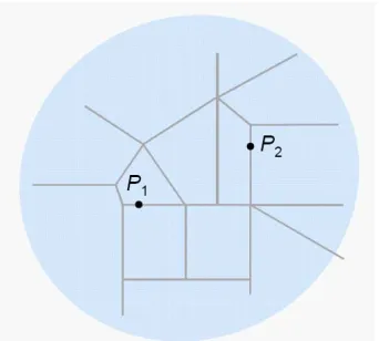
Figure 3.6: Location update from

P1

to

P2

leaves ambiguous paths

... 63

Figure 3.7: Raw location points, candidate for a trajectory leg.

... 64

Figure 3.8: Proposed algorithms on the raw points would yield mobile user’s trajectory

... 65

Figure 4.1: GIS General Architecture

... 68

Figure 4.2: GIS data layers

... 69

Figure 4.3: Representation of a point and a line in vector and raster format

... 70

Figure 4.4: ArcGIS Architecture

... 70

Figure 4.5: A logical model of a road

... 72

Figure 4.6: Vector modeling of a road network

... 73

Figure 4.7: GIS database creation from different sources

... 75

Figure 4.8: Two modes of manual digitization, point and stream modes

... 77

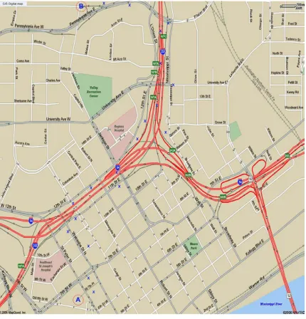
Figure 4.9(a): Paper map of urban area to be digitized for GIS database

... 78

ix

Figure 4.10: Geometric Point-to-Point matching

... 81

Figure 4.11: Point to Curve matching issue (1)

... 82

Figure 4.12: Point to Curve matching issue(2)

... 82

Figure 4.13: Problem with Curve-to-Curve matching

... 83

Figure 4.14: Improving Point-to-Curve matching

... 84

Figure 4.15: Fréchet distance famous man dog example

... 89

Figure 4.16: Mobile Trajectory Based Services Architecture

... 90

Figure 4.17: Road network element model

... 92

Figure 4.18: A logical representation of topology of metric space. Metric (distance) is defined

between any two points. The distance is through the connected points.

... 96

Figure 4.19: A parametric representation of a road element in topological space

... 99

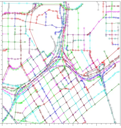
Figure 4.20: Topological representation of road map of an urban area. Roads are represented

by connected and intersecting polylines. Polylines are expressed in vertices shown as

squares.

... 100

Figure 4.21: The triangle inequality scenario 2, when the three locations are not

... 101

necessarily on the same road.

... 101

Figure 4.22: Straight lines through some vertices outside the error ball may pass through it .. 111

Figure 4.23: The corrected location must lie between the two vertices for the geodesic to be

candidate geodesic

... 115

Figure 4.24: Vehicle heading from L

1

to L

2

wrongfully matches the road segment s

1

... 118

Figure 4.25: In both the projection scenarios

SE

is selected as the candidate segment

... 118

Figure 4.26:

V V

_{1 2}

is a candidate geodesic in an error circle of radius r centered at (h,k)

... 119

Figure 4.27: An example of geodesic candidate selection

... 120

Figure 4.28: The next position of the error ball is estimated at the nearest intersection from

the corrected locations.

... 122

Figure 4.29: Selection of next intersection in a grid-like road network

... 126

Figure 4.30: Selection of next intersection in a directional road network

... 127

Figure 4.31: Selection of next intersection in a two-way road network

... 128

Figure 4.32: Illustration of direction of transition of an error ball,

α

, the direction difference

off set,

θ

,and difference error,

β

.

... 129

Fig. 4.33: Logical partitioning of trajectory

... 132

Fig. 4.34: Direction negativity and path constrains on error ball and its image

... 133

Figure 4.35: Map-matching of pre-matched curve with the set from GIS database

... 133

Figure 4.36: Trajectory estimation flow chart

... 134

Figure 4.37: MTBS provisioning

... 135

Figure 4.38: MTBS protocol flow

... 136

Figure 5.1: Digitizing table acts as an input source to a computer

... 137

Figure 5.2: Digitizer’s GUI

... 138

Figure 5.3: Map image loading into Digitizer

... 139

Figure 5.4(a): Zoom feature of the Digitizer

... 140

Figure 5.4(b): Digitized roads and application of unification

... 141

Figure 5.5: Reconstruction of road network map of Figure 4.9(a) from database

... 142

x

Figure 5.7: Map of Figure 4.9(b) reconstructed from database

... 143

Figure 5.8: Database points are represented with squares

... 144

Figure 5.9: Location estimation simulation model

... 145

Figure 5.10: Error simulation in digital map

... 145

Figure 5.11: Mobility Profiling simulator’s GUI, the mobility simulation window

... 146

Figure 5.12: Mobility profiling simulator’s GUI, the trajectory estimation window

... 148

Figure 5.13: Mobility profiling simulator window with reference map

... 149

Figure 6.1: Anomaly in Fréchet distance

... 152

Figure 6.2 (a): Result with location error of 25m

... 153

Figure 6.2(b): Result with location error of 50 m

... 153

Figure 6.2 (c): Result with location error of 75 m

... 154

Figure 6.2(d): Result with location error of 100 m

... 154

Figure 6.2 (e): Result with location error of 125m

... 154

Figure 6.2(f): Result with location error of 150 m

... 154

Figure 6.2 (g): Result with location error of 175 m

... 155

Figure 6.2(h): Result with location error of 200 m

... 155

Figure 6.3: En error of 200m yields higher trajectory error using dense part of the map

... 156

Figure 6.4(a): Trajectory estimation error vs. Location estimation error of different

technologies

... 157

Figure 6.4(b): Linear and Areal Error Ranges

... 157

Figure 6.5 (a): Suburban Trajectory estimation with 100 m error

... 158

Figure 6.5 (b): Suburban Trajectory estimation with 200 m error

... 158

Figure 6.5 (c): Suburban Trajectory estimation with 400 m error

... 159

Figure 6.6(a): Example 1 of Global Map-Matching accuracy in mobile network

... 161

Figure 6.6 (b): Comparison run of example 1 in Figure 6.6(a), using our proposed method.

.. 162

Figure 6.7(a): Example 2 of Global Map-Matching accuracy in mobile network

... 162

Figure 6.7 (b): Comparison of example 2 in Figure 6.7(a), using our proposed method.

... 163

Figure 6.8(a): Example 3 of Global Map-Matching accuracy in mobile network

... 163

Figure 6.8 (b): Comparison of example 3 in Figure 6.8(a), using our proposed method.

... 164

Figure 6.9(a): Error comparison in terms of Fréchet distance

... 165

Figure 6.9(b): Error comparison in terms of Average Fréchet distance

... 165

Figure 6.10(a): Statistics of the comparison simulations (Fréchet distance

... 166

Figure 6.10(b): Statistics of the comparison simulations (Average distance

... 166

Figure 6.11: Trajectory1: Trajectory used to collect location data set 1 and corresponding

matching result

... 168

Figure 6.12: Trajectory2: Trajectory used to collect location data set 2 and corresponding

matching result

... 168

xi

LIST OF TABLES

Table 2.1: LBS and the required location accuracy

... 42

Table 2.2: Upper layers services in MLP

... 54

Table 3.1: Location estimation technologies’ accuracy comparison

... 62

Table 4.1: Parameters of a road element

... 93

Table 4.2: Definition of the road from end to end

... 94

Table 4.3: Example of the road parameters from database to be used in simulation

... 94

Table 4.4: Example of the road definition from database to be used in simulation

... 94

Table 6.1: Performance Comparison with no Node Buffer

... 170

Table 6.2: Performance Comparison with 10m Node Buffer

... 170

Table 6.3: Performance Comparison with 20m Node Buffer

... 170

1

Chapter 1

Introduction

The location specific services came to usage with the deployment of NAVSTAR GPS (Navigation

Signal Timing and Ranging Global Positioning System), commonly called, Global Positioning Systems (GPS), by the US Department of Defense in the 70’s. Initially the services were exclusively for military purposes. In 1984 the US government granted GPS civilian access, however with an intentional error, called selective access. In May 2000, selective access was removed and the civilian began enjoying relatively lower error positioning systems [1]. Within the last few years there has been a massive surge of interest in yet another positioning methodology and applications that could use the positioning information using cellular networks and handsets. The reasons for this surge is mainly because new wireless positioning technologies have the capability of alleviating the shortcomings of GPS, such as high power consumption, slow-to-acquire initial position, and legislation in the United States requiring cellular phones operators to provide location information to 911 call centers. A large proportion of the 911 calls come from cellular phones. The FCC mandate (docket 94-102) [2] requires mobile network operators to provide positional information to emergency services accurate within 125 meters. This regulatory requirement provided a stimulus for the commercial development of wireless positioning technologies and applications built on them, hence the birth of location based services (LBS). Mutual advances in location determination and geo-spatial technologies have provided a rich platform to develop mobile LBS [3]. Within the context of LBS, mobile wireless communication and geo-spatial database go hand in hand.

2

LBS are locating the nearest point of interest (directory assistance), navigation aids, security, advertisement, dating, location specific promotion, safety, and entertainment. We shall cover LBS in greater detail in the following chapters.

In a mobile network, the user’s location information, in x-y coordinates on a map, is determined by any given location determination technology, such as time of arrival (TOA), time difference of arrival (TDOA), angle of arrival (AOA), time advance (TA), Cell-ID, and assisted-GPS (A-GPS). These technologies usually require modifications in either the networks or the mobile phones, and in some cases, in both. LBS have generated a lot of interest in recent years, as a new source for mobile operators to enhance their service offering, thus potentially increasing revenues. LBS are achieved with the exact information of a user’s location in real time with personalized setup and location sensitivities. These services are based on wide range of accuracies of the location. Some services may require an almost exact position, whereas others can be built on RF segment, cell, or even location area (several cells) information. However, all such services are based on points (exact locations) and areas (cell or location areas, city, or even country).

We focus on the methodology that could provide location services that are based on the exact trajectory (mobility profile) of a mobile user. This is a new area of research. We investigate suitability of underlying location determination technologies. The challenge is the location accuracy. It is very improbable to generate a user’s exact trajectory with a high-error underlying technology like TA, or even some implementations of TOA and TDOA. There is a plethora of services that could be based on the information on the mobility profile of a user. Mobility models studied in the literature and some used in location management (IS-41) can do very little to develop a mobility model for each individual user. The logical approach is to use the mobility traces.

3

Mobility profiling gives birth to a new direction in LBS; we called them Mobile Trajectory Based Services (MTBS). These services are based on spatiotemporal distribution. Each point is the distribution of the form (x,y,t), where x,y are location coordinates and t is the time stamp associated with the location. MTBS could use a user’s trajectory of the day and estimate where the user is likely to be, on the trajectory at some future times. For this reason, some of these services could be referred as Future Location Based Services (FLBS). For a comparison between LBS and MTBS for the same service, consider the following example: You are passing by a Sears department store and you receive a soft promotional coupon on your phone from the store. They are offering you a matching shirt to a jacket you bought some time ago. However, with MTBS the same service could be extended well in advance. A similar coupon could be solicited while you are on the beginning of the trajectory, or even while you are still at home. Some MTBS can be built on just the spatial part of a trajectory, for example, optimal path suggestion. Figure 1.1 shows a conceptual comparison of LBS and MTBS.

Figure 1.1: A conceptual comparison of LBS and MTBS

1.1

Challenges in Mobility Profiling

4

Collectively, TOA, TDOA, and; OTD are referred to as time-based methods. In TOA, the network measures the time of receipt of a transmission from the mobile. This time is measured at three or more base stations. The network can convert these times into distances and triangulate on the result. Time difference of arrival (TDOA) has been the preferred technology of choice for high-accuracy location systems since the advent of radar. TDOA systems operate by placing location receivers at multiple sites, geographically dispersed in a wide area; each of the sites has an accurate timing source. The differences in time stamps are then combined to produce intersecting hyperbolic lines from which the location is estimated. The most popular method to estimate TDOA is through the use of cross-correlation, in which the received signal at one base station (BS) is correlated with the received signal at another BS. The global positioning system is a TOA-based system, as are most of the systems proposed for the Location and Monitoring Service (LMS) band recently allocated by the FCC. However, the position estimation is done in the handset. It is referred as OTD (Observed Time Difference). OTD relies on installing location management units (LMUs) at known locations that can measure signal timings from cells. The signal timings from a minimum of three cells to the device are also measured. These timings can be combined to work out the distance of the user from each of the cells. This distance can then be used to triangulate a position.

5

the true location, is called map-matching. Our assumption is that a mobile user travels on roads. Map-matching maps the estimated raw location point to a point on the road network, or it could map the whole curve, consisting of erroneous estimated location points, to a set of roads on the digital GIS map which corresponds to the mobile user’s true trajectory. This method of map-matching is referred to as curve-curve matching. GIS is an integral part of the mobile wireless LBS infrastructure [4]. GIS and map-matching are introduced briefly in the following sections.

1.2

Geo-spatial Technology in LBS

The very nature of LBS makes geo-spatial technologies a necessary element. The geo-spatial technology used in LBS is called GIS. GIS has been used in all disciplines of life that have any relation to geo-spatial data. GIS is a system for creating, storing, analyzing, and managing geo-spatial data and the associated attributes [5]. In the strictest sense, it is a system capable of integrating, storing, editing, analyzing, sharing, and displaying geographically-referenced information, see Figure 1.2.

Figure 1.2: GIS high-level architecture

6

Figure 1.3: High level GIS layers representation

Some features can appear in multiple layers. For example, a street can also be a ZIP code boundary and a city boundary line. The street could then appear in three layers: one containing the streets, one containing the ZIP code boundaries, and one containing the city boundaries. In our work we are interested in the layer that models and depicts road networks. The roads are modeled as polylines or arcs [7][8]. Arcs are represented with starting and ending nodes, which imparts directionality to the arcs. The arcs pass through several vertices along the way. Each of the nodes and vertices are stored with coordinate values representing real-world locations in a real-world coordinate system, such as longitude/latitude angles, State Plane feet, or Universal Transverse Mercator (UTM) meters. These coordinate values represent locations you could locate using the numeric values printed on the graticule on the edges of a paper map. Along with, direction of a road, other important associated information like speed and direction, is also available. The constraints of direction and speed further help in the decision-making of map-matching. GIS is discussed in details in the following chapter.

1.3

Location Comparison with Map

The estimated location is compared with a map through a process called map-matching. Map-matching is defined as the process of correlating two sets of geographical positional information, for example location records of object positioning, from different location determination techniques, to the points on digital road networks from a digital map of a GIS. Data types handled by map- matching include point-to-line, line-to-line, and polyline-to-polyline matching [9]. Based on the temporal-response characteristics, map-matching algorithms can also be roughly classified into online map-matching and off-line map-matching. Online map-matching methods snap an estimated location to the base reference in real-time. Offline map-matching counterparts post-snap the point

Digital Orthophoto Roads Hydrography

Parcels Buildings

7

data or linear data after the whole set of data is collected. We shall do online map-matching for point-to-line and offline map-matching for curve-to-curve (or ployline-to-polyline) matching.

1.4

Proposed Mobility Profiling

Mobility profiling, within the context of MTBS, is a set of mobility traces of a mobile user for all of the days of the week. During the profiling week, the mobility traces are generated upon which the MTBS are built.

Polling the current locations of a mobile user to collect the estimated location points is adaptive and depends mainly on the topology of the road segments on which the mobile user is potentially traveling. Each road in the GIS database is associated with a direction and maximum speed limit.

Since there is an error, ε, associated with the estimated location, the mobile user could be on any road

segment contained in a circle of radius ε with center at the estimated location coordinates. This is how we perform mobility profiling: 1) Map-match the raw location point to all of the potential location points on the road within the error circle.

2) For each road, find the next node, (that is the road turn) and estimate the time, ttp, to reach the turning point. Pick the nearest turning point and do the next poll at ttp

3) Eliminate the road segments from the candidate roads pool in the error circle using direction and speed, GIS constraints. During the profiling time, the mobile user is moving for some of the time and is at rest for remainder of the time. This yields a spatiotemporal distribution with clusters, the clusters being the rest positions. A trajectory leg is from one cluster to another.

. If we have only one road in the error circle, that is the exact road; if we have more than one, then each road is a potential candidate.

8

1.5

Contributions and Organization of the Thesis

This thesis focuses on mobility profiling of a mobile user in an erroneous environment of cellular network systems, emphasizing the implementation aspects. It contributes with the introduction of MTBS and the advancement of the trajectory estimation method suitable for MTBS. The contributions are summarized below.

1.5.1

Introduction of MTBS and Their Provisioning Architecture

E911 gave birth to the services based upon the known location of a mobile user, i.e., LBS. We introduce the idea of Mobile Trajectory Based Services that are based upon the known mobility pattern of a mobile user. The mobility pattern is available to the mobile service providers in the system’s database, which was profiled a priori. The effectiveness of MTBS and a comparison with LBS is described in Chapter 3. A system-level architecture of mobility profiling, the MTBS protocol, and provisioning are introduced and explained at the end of Chapter 4.

1.5.2

Road Network and Mobile Trajectory Framework

9

going in the opposite direction of the road, yet not exactly at a difference of 180. A direction negativity condition is defined to compare the directions of a path on a road network and the transition of the error ball. The details of all of these contributions are given in Chapter 4.

1.5.3

MAP Digitizing Software Application

The GIS database of a road network plays a pivotal role in trajectory estimation. The GIS database for road networks is available, but the software packages to access the database, such as, Arcview, from ESRI are very expensive, only affordable by a corporation. We decided to digitize the paper maps ourselves. To digitize paper maps into digital maps, one requires a digitizing table which interfaces with a PC to store the digital version of the map. We designed an application (we called it Digitizer) that would load any given map in an image form, and with mouse clicks on the roads on screen generates the digital version of the map. We can assign road attributers for each digitized road. So, essentially it is a software version of the digitizing table. Hand error, which is the main source of error in digitizing a map, is alleviated with the Digitizer, because one can zoom into the map to see the road lines thicker and work in the center of the lines, which we cannot do with the digitizing table. A small hand error is fully absorbed within the relatively large width of a road. This makes digitization efficient and increases the resolution tremendously. The zoom effect can further be enhanced by lowering the screen resolution.

1.5.4

Mobility Profiling Algorithm and Simulation

10

published trajectory estimation method, called Global Map-matching, using its performance metrics. The results of our simulations and that of the comparison are given in Chapter 6.

1.5.5

Organization of the Thesis

11

Chapter 2

Location Estimation Technologies and Location

Based Services

The realization of LBS can be described by a three-tier communication model including a location layer, a middleware layer, and an application layer. All three layers may require access to geo-spatial data. The model is shown in Figure 2.1. The location layer is responsible for calculating the location of a mobile device or user. It does so with the help of underlying location determination technology and geospatial data held in a Geographic Information System (GIS).

Figure 2.1: LBS communication model

While the location determination system calculates where a device is in network terms, GIS allows it to translate this raw network information into geographic information (longitudes and latitudes). The end result of this calculation is then passed on via a location gateway either directly to an application or to a middleware platform. Originally, the location layer would manage and send location information directly to an application that requests it for service delivery. The application layer (which in the LBS industry is often and confusingly referred to as a "client") comprises all of those services that request location data to integrate it into their offering (for example, a friend finder); however, as increasingly

more LBS applications are being launched, many network operators have put a middleware layer

12

complexity of service integration because it is connected to the network and an operator's service environment once and then mitigates and controls all location services added in the future. As a result, it saves operators and third party application providers, time and cost for applications integration.One can think of LBS processes consisting of two main parts:

1) How a device can get its geographical location information and send it to an application server (such as a Web server). This is the core of LBS. In the next generation of wireless communications (3G or UMTS) [11], these additional entities and mechanisms are standardized and they are known as Location Services (LCS) [12].

2) How the server can use the provided geographical information and either return the appropriate response or activate relevant operations according to the service query. This response should include the relevant service information requested by the user, such as “where is the restaurant, nearest gas station, nearest printer?” and so on.

In our literature survey, we focused on both of the above parts of LBS. There are different solutions for implementing LBS and they comprise both wired and wireless technologies. The wireless communications are moving towards IP networks to provide unified communications across wired and wireless boundaries. This is the All-IP system, which provides seamless integration of communication services and Internet applications.

2.1

LBS System Architecture

13

Figure 2.2: End-to-End LBS system architecture

In rest of this chapter we shall cover all three layers in detail and conclude with key protocols for LBS.

2.2

Location Estimation Technologies

Throughout time people have developed a variety of ways to figure out their position on Earth and to navigate from one place to another. Early mariners relied on angular measurements to celestial bodies like the sun and stars to calculate their location. The 1920’s witnessed the introduction of a more advanced technique—radio navigation—based at first on radios that allowed navigators to locate the direction of shore-based transmitters when in range. Later, the development of communication satellites made possible the transmission of more-precise, line-of-sight radio navigation signals and sparked a new era in navigation technology. Satellites were first used in position-finding in a simple but reliable two-dimensional US Navy system called Transit. This laid the groundwork for a system that would later revolutionize navigation forever—the Global Positioning System.

14

calls per day placed from cellular telephones alone, about 25% of all such calls placedannually. This has resulted in the FCC E911 mandate (docket 94-102) that requires mobile network operators to provide positional information to emergency services that is accurate to within 125 meters [14-17]. This regulatory requirement has provided a stimulus for the commercial development of wireless positioning technologies and applications built on to those technologies.

A cellular-based location takes advantage of the existing transceivers, communication bandwidth, two-way messaging, and well established infrastructure, but also inherits the disadvantages imposed by the design of the communication systems [18]. There are several technology alternatives for locating cellular telephones. If one considers modifications to the telephone, GPS is the most commonly discussed option. For locating unmodified cellular telephones, signal attenuation, angle of arrival (AOA), time of arrival (TOA), time difference of arrival (TDOA), enhanced observed time difference (E-OTD), and time advance (TA) are used. All technologies are based on knowing the locations of existing reference points (GPS satellites, cellular radio base stations) and then relating them to the location of the mobile station. The signal strength method has not received as much attention as most of the other methods have, but some remarkable results have been reported [19]. AOA and TDOA are the most discussed methods. AOA was first developed for military and government organizations, because it operates with no modification of a mobile device, and was later applied to cellular signals. It is based on the estimation of the mobile station (MS) signal angle at the base stations (BSes). It requires an array of antenna elements. Future wireless systems may have more sophisticated and intelligent antenna systems [20]. The time-based methods, TOA, TDOA, and OTD, work on the basis of the time a signal takes in propagating from one place to another, from the MS to the BSes in case of TOA, and from BSes to the MS in the case of OTD. Because of the fact that in TDMA the system knows how much time a signal takes to reach the MS, TDMA is also exploited for location estimation. However, a large error is associated with this method [21]. For handset modification, a GPS-assisted method is most desired; however, millions of handsets are in operation already, therefore non-GPS methods are under highly motivated research and development.

15

location technologies. Irrespective of which underlying principle is used, the final product must achieve an accuracy of better than 125 meters. This requirement is a direct outcome of the FCC (Federal Communications Commission) mandate r to make emergency management more effective.

It is unlikely that any one system (TOA, TDOA, E-OTD, or AOA etc.) will be able to provide accurate mobile positions under all circumstances [23]. The final solution to this problem is a more pragmatic combination of several location methods working together. TOA is expected to make a significant contribution to such a combined solution.

2.2.1

Time-Based Methods

16

2.2.1.1

Time of Arrival

TOA, a popular radio location technique, is based upon the measurement of the arrival time of a signal transmitted from the MS to several (at least three) BSes. The distance between the MS and the receiving BS is determined from the time the signal takes from the MS to the BS. The distance is cT, where c is the velocity of light and T is the time of travel from MS to BS. Geometrically, it represents a circle of radius cT, on which the BS must lie. Figure 2.6 shows three BSes, BS1, BS2, and BS3, receiving the signal from the MS, at times T1, T2, and T3 respectively.

To determine the location of the MS, three circles of radii cT1, cT2, and cT3 are drawn, with centers at the respective base stations, where T1, T2, and T3 are the times, the signal (a sequence) took to travel from the MS to the BS1, BS2, and BS3 respectively, as shown in Figure 2.3.

Figure 2.3: Location estimation with TOA

17

The disadvantage of this technique is that the MS must behave like a transponder [27][28]. The processing delays and non-LOS propagation (multi-path propagation) can cause errors, hence an inaccurate TOA estimation. In this situation the geometrical approach is difficult. The circles may not meet at one point. One approach is to estimate TOA based on the transmission of one known data burst, such as a midamble in a GSM normal burst. For a sufficiently short burst, the channel can be represented as a time-invariant multipath channel. The channel consists of a linear combination of time-delayed Dirac delta pulses with amplitude amand delaysτm

), ( . ) ( 1 m m M m

ch t a t

h =

∑

δ

−

τ

=

.

(2.1)

where each Dirac delta pulse represents one multipath component. If the channel impulse response contains a line of sight (LOS) component, the minimum overall τm refers to the TOA, from which the MS distance from the BS is determined.

Another approach is to estimate the position using a non-linear least-squares solution [23][28]. An MS at(x y0, 0), transmits its burst at

τ

0. The locations of the N BSes are represented as

1 1 2 2

( ,x y ),(x y, ),...,(xN,yN). They receive the sequence at time τ τ1, 2,...,τN .

2 2

(x) ( ) ( ) ( )

i i i i

f =cτ τ− − x −x + y −y

. For performance measure a function:

(2.2)

is defined, where c is the speed of light and x=( , , )x yτ T. With the proper choice of, x y, andτ , (x)

i

f formed at all of the BSes could be made zero. However, the measured TOA values are not

error-free,due to multipath and other impairments. Under unconstrained non-linear least-square approach, the function: 2 2 1 (x) (x), N i i i

F a f

=

=

∑

(2.3)

where '

i

a s are the reliability weights of the signal reception at the BSes. The location estimation is

achieved by minimizing the functionF(x). The steepest descent method can be used to solve the above mentioned non-linear problem. The successive locations are updated according to the following equation:

1

( ),

k k x k

18

whereμis a constant , T

( x , y ,_{k k k})

k

x

= τ

,

dx d x≡ ∇ and

|

|

(

)

( ) |

|

k k k k x y x z x _k

F

x

F

F x

xf x

y

F

z

∂







_∂







∂





∇

= ∇

_{= }

_

∂





∂







_∂







(2.5)

The constant μis chosen small enough for the convergence. The recursion continues until

1 |

|

x

k+ −

x

k reaches an accepted minimum value. However, it might take a long time to converge, or

it might not converge at all if the minimum accepted error is small. Another method is proposed in [28] to solve (2.3) by linearizing fi(x) with Taylor Series expansion about xk

( ), 1, 2,... ,

i i

r =c

τ τ

− i= N

keeping only the first order term. Putting a constraint on the non-linear least-square solution, with the fact that the range error is always positive, we get an area of MS location. This is because the TOA estimates are always greater than the exact true TOA values, due to multipath and non-LOS propagations plus other impairments. Therefore, the true location of the MS must lie inside the circles of radii

about the N BSes. Since the MS cannot lie farther from a BS than its corresponding range estimate, the location of the MS can be represented as the shaded area in Figure 2.4.

Figure 2.4: Location feasible area

19

inequalities:

2 2

(

)

(

)

(

)

i i i i

r

=

c

τ τ

−

≥

x

−

x

+

y

−

y

for i = 1,2,3. (2.6)

This implies:

2 2

(

x

_i

−

x

)

+

(

y

_i

−

y

)

−

c

(

τ τ

_i

−

)

≤

0.

(2.7)

Here g x_i( )= −f x_i( ).This leads to the restrictions f x_i( )≥0.The constraint boundaries form the

feasible area.

There are many approaches to forming numerical solutions for the constrained in (2.7). One of them uses penalty functions to modify the objective function in (2.3):

[

]

1

2 2

1 1

( ) ( ) ( )

N N

i i i

i i

F x a f x P g x −

= =

=

∑

−

∑

(2.8)

P is a positive quantity. The penalty functions provide a large penalty to the objective function when one

or more constraints are violated. The search procedure is the optimization of a sequence of surfaces toward the true value of the objective function. Initially, an unconstrained search method is used to

provide an artificial optimum x1 with a large value ofP=P1. The next stage is initialized with the

previous estimates x1 and uses a smaller P=P2 to provide a better approximation to the true optimum.

The solution is discussed in detail in [28]. [29] proposes a residual weighting algorithm, to mitigate the NLOS errors.

This algorithm assumes that the number of range measurements is greater than the minimum required. [30] introduces a sub-optimal maximum likelihood estimation algorithm that maximizes the signal-to-noise ratio gain at the output. This approach is similar to TDOA, mentioned in the next subsection. [31] suggests TA of TDMA systems for the estimations of TOA. TDMA systems measures TOA with a certain raw measurement error. TA is assigned from this to one of the finite sets of values, resulting in a multitonial distribution of results. It is assumed that the user does not have access to the original TOA measurement and must attempt to reverse the process and estimate the TOA from the TA. The resultant error in the estimated TOA might be large if the wrong TA bin has been selected. This solution improves the accuracy of TOA by taking the average of two or more consecutive TA values.

2.2.1.2

Time Advance

20

base station, carries the cell identity. This location area can be further narrowed with the time advance (TA) feature. In TA, a TDMA cell knows the time it takes for its signal to reach a mobile device. This knowledge is required because multiple devices share the air interface at the same frequency using different time slots (TSes). To ensure that the signal from a device that is distant from a cell does not stray outside its TS, a TA signal is sent to the MS. This ensures that the time taken for the signal to travel from the device to the cell is taken into account. This TA signal can be converted into a distance. The distance has a precision of 550 meters, thus providing a location that looks like a “doughnut” (Figure 2.5). In an urban area, this may be acceptable, especially if directional antennae are taken into account. Precision in a rural area will be poor.

Figure 2.5: TA compared with other legacy location techniques

21

Because of the error associated with the propagation time by the BS [21], this method is not considered the primary method for position estimation. This is considered a good fall-back method, in case the primary method fails for some reasons associated with the primary method.

2.2.1.3

Time Difference of Arrival and Observed Time Difference

TOA requires that all of the BSes and the MS have a very precise synchronized clock, and the transmitting signals be labeled with the time stamps. Moreover, the MS must behave as a transponder that has a high potential of processing delays and non-LOS errors. Just one microsecond of timing error would cause 300 meters of location error. For these reasons, TDOA measurements are a more practical means of determining location for commercial systems [22], and are now considered the leading candidate for future location estimation systems [33].

TDOA determines the position of the MS by examining the difference in time at which the signal arrives at multiple BSes, rather than the absolute arrival time. If the BSes are at the two focii of the hyperbola, the mobile station must lie on the hyperbolic curve. By drawing two such hyperbolas with two sets of BSes (total minimum of three BSes), the intersection would determine the MS location. Both uplink and downlink TDOA methods have been proposed. In the latter case, it is referred to as OTD, as shown in Figure 2.6.

Figure 2.6: Location estimation with TDOA

22

At least three BSes must transmit a very accurate clock time value to the MS. The MS sees three different clock times which are “behind” the real network time by an amount that depends on the times the clock values have taken to travel to the MS. The MS examines these times in pairs. For any particular pair of base stations, the difference in the time is related to the difference in distance to those two base stations. It is therefore possible to draw a line of constant difference of distance, a hyperbola. If the mobile receives signals from three BSes, then it can draw three hyperbolas as shown in Figure 2.6.

In a GSM implementation of OTD, pseudo-synchronous handover is supported in the MS. The timing accuracy in this case is well below a bit period. This is referred to as Enhanced-OTD [26]. In GSM, the BSes are not synchronized. Instead, location monitor units are used to determine the time of launch of the signals from each BS. Motorola’s iDEN system also uses OTD. The synchronization between the BSes is achieved through GPS receivers [34]. This ensures that the BSes broadcast each TS at approximately the same time.

As already mentioned, in OTD the measurements of propagation time are not used directly. The OTD is the time interval between the receptions of bursts from two different BSs, i.e., if bursts are received at t1and t2at the MS from BS1 and BS2 respectively, OTD = t2−t1, assuming t2>t1 . If

the BSes are not synchronized, a parameter called, RTD (Real Time difference) is taken into account. The RTD is the difference in the burst transmit time, i.e., if at BS1 the burst is transmitted at t3 and

at t4 at BS2, RTD=t4−t3, assuming, t4 >t3. In a synchronous network, the RTD is zero. To

describe the geometrical effects on the burst reception time, [35] defines the GTD (Geometric Time Difference) as follows:

2 1_,

d d

GTD c

− =

where d1 and d2 are the displacements (propagation paths) of BS1 and BS2 to (or from) the MS

23

thus the hyperbolic belts, represents the possible positions of the MS. The intersection of two such hyperbolas represents the feasible area of the MS. The feasible area could be reduced by using more GTD values from other sets of BSes.

The same treatment is true for the TDOA, the only difference being that the estimation is done on the location processing system, which takes the TDOA values from the BSes. Since TOA and TDOA are two independent methods, they can be used together to enhance the precision of the location estimation. [36] uses such an approach.

Obtaining the MS position from TDOA is a two-stage process. In the first stage, accurate estimates for the TDOA values are computed from the noisy signal. In the second stage, potentially inconsistent and noisy estimates are processed to determine the location.

The most widely used method to estimate the TDOA is called generalized cross-correlation

[32-33][37-40]. The TDOA is the delay that maximizes the cross-correlation. The general model for estimation assumes that the arriving signals have the following form:

1( ) ( ) 1( ),

r t =s t +n t (2.9)

2( ) ( ) 2( ),

r t =

β

s t− +

τ

n t (2.10)

where

τ

is the delay (TDOA) of the signal received at the BS2 with relative to BS1. s t( ) is the original signal, n t r t₁( ), ( )₁ and n t r t₂( ), ( )₂ are the uncorrelated zero-mean Gaussian noise, and the

received signals, at BS1 and BS2 respectively.

β

is an attenuation factor. The signal received at both of the BSs are of the form r t( )=

β

s t( − +

τ

) n t( ),however r t₂( ) in the (2.10) is relative to r t₁( )in (2.9). The cross-correlation of (2.9) and (2.10) is given by

1,2 1 2

0

1

( )

( ) (

)

T

C

r t r t

dt

T

τ

=

∫

−

τ

(2.11)

SNR (Signal-to-Noise Ratio) in this estimate could be improved by increasing the integration interval, T, the time of observation. The TDOA,

τ

TDOA, is the

τ

, with a peak in C1,2( ).

τ

The cross-

24

In a CDMA system, a PN (Pseudo Noise) code synchronization module is used to acquire system time and to perform synchronized demodulation. Its function includes PN code tracking within 1 chip period. [41] proposes the use of pilot signals to calculate TDOA during PN code synchronization. However, this would require a slightly modified MS, either through hardware or software. This is true for all OTD-based solutions.

In generalized cross-correlation, r t1( ) and r t2( )are pre-filtered prior to cross-correlation for

improved accuracy of the

τ

TDOA. Smooth coherence transform, maximum likely, Hassid-Boucher,

and the Wiener processor are the examples of such well known filters. The justification for filtering can be given as follows: Cross-correlation in (2.11) can also be represented as:

1,2( ) 1,2

j f r

C

τ

U eπ τdf

∞

−∞

=

∫

(2.12)

where C1,2( )

τ

is the cross-power spectral density function. After r t1( )and r t2( )are filtered prior to

cross-correlation, to produce, for example f t₁( )and f t₂( ) respectively, then the cross-power spectral density becomes:

*

1,2

( )

1

( )

2

( )

1,2

f

U

f

=

H f H

f U

(2.13)

where H1( )f and H2( )f are the transfer functions of the filters used to filter r t1( )and r t2( )

respectively and * denotes complex conjugate. Therefore, the generalized cross-correlation can be expressed as:

* 1,2

( )

1,2 1

( )

2

( )

j f

f f

C

τ

U H

f H

f e

π τ

df

∞

−∞

=

_∫

(2.14)

By properly choosing *

1( ) 2( )

H f H f , i.e., proper filtering, the effect of noise and interference could

be reduced. Figure 2.7 shows a generalized cross-correlation method. The output D

∧

25

Figure 2.7: Generalized Cross-Correlation method

[38] introduces a novel thresholding technique, wavelet demising. The demising technique is a three-step process. First, taking wavelet transform of the received signal, thresholding the wavelet coefficients and then performing the reverse transform of the modified coefficients. Wavelet transform is the transformation of the received signal into two wavelets, one of the source signal and the other of noise. These wavelets are in matrices form. The source signal wavelet has many small magnitude terms (coefficients), which are adjusted in the thresholding rule. The filtering techniques do reduce the effects of noise and interference on TDOA, but multipath anomaly can still cause problems in generalized cross-correlation. This is due to the fact that overlapping cross-correlation peaks often cannot be resolved. A method to identify and select the right peak, needs to be devised such as selecting he first peak or largest peak. There has been significant research into applying the theory of cyclostationary signals to improve the resolution of the generalized cross-correlation method [32]. This would improve performance in multipath environments. In an impulsive environment, generalized cross-correlation, which is based on the assumption of finite noise variance, would not give a reliable TDOA. Using the theory of J-stable distributions, [42] developed several robust algorithms to tackle this issue. However, these algorithms assume a static and multiple of sampling interval delay. By expanding this idea along with [43], a simplified explicit time delay estimator, [44] developed an adaptive algorithm which can track time-varying delays of any real values under stable noise conditions. This is an iterative least mean square method which converges fairly quickly, in 2000 iterations.

After the TDOA has been estimated, the range difference is calculated. The range difference between BS1 and BS2:

1,2 2 1 TDOA2,1.

r = − =r r c

τ

(2.15)

Let ( ,x y1 1) and (x2,y2)be the coordinates of BS1 and BS2 and those of the MS be (X,Y). The

26

2 2 2 2

2,1 ( 2 ) ( 2 ) ( 1 ) ( 1 ) .

r = x −X + y −Y − x −X + y −Y (2.16)

Similarly, for an estimated TDOA between another set of BSes, such as BS2 and BS3, (2.15) and (2.16) could be rewritten as:

2,3 3 2 TDOA3,2

r = − =r r cτ (2.17)

2 2 2 2

3.2 ( 3 ) ( 3 ) ( 2 ) ( 2 )

r = x −X + y −Y − x −X + y −Y (2.18)

By solving equations (2.16) and (2.18) (X,Y,Z) is found. Its geometrical representation is shown in Figure 2.6. [45] and [39] show a complete solution of such equations. The latter solves these equations for 4 BSes. [46] gives the solution for E-OTD.

As noticed in equations (2.16) and (2.18), by choosing the BSs sets as BS1,BS2 and BS2,BS3, the solution is relatively easy. However, the solution becomes more difficult when BS sets are arbitrary, which is more typical in PCS and cellular environments. One of the solutions is to linearize the equation through Taylor series expansion, ignoring the higher order terms. However, it could result in significantly erroneous location coordinates under some situations, due to geometric dilution of precision (GDOP). This is very much dependent on the cell layout topography [47]. In this situation a relatively small

τ

TDOAwould result in a large position location error because the MS is located in the

hyperbolic curve far away from the focii, i.e., the BSes. TDOA gives very accurate results if the MS is located between the BSes. [48] gives a closed-form solution valid for both, distant and close sources, and is an approximation of the maximum likelihood estimator when the TDOA errors are small. This solution provides excellent results on arbitrarily distributed BSes, tolerable to a higher noise threshold, and performs better than most of the solutions, including Taylor series approximation. In this method, an intermediate variable transforms the non-linear equations into a set of equations which are linear in the MS coordinates and the intermediate variable. An intermediate solution is found using least the square method. By exploiting the known relationship of the intermediate variable with the position coordinates, the final solution is computed.

2.2.2

Angle of Arrival

27

position of an MS is estimated from the angles of the incoming signals detected at the fixed BSes, as shown in Figure 2.8.

Figure 2.8: Location estimation with AoA

In general, the antenna elements are spaced on the order of half the wavelength of the carrier frequency. The relatively close spacing of the antenna elements allows the time delays seen by a signal as it propagates across the array to be modeled as phase shift. This narrow-band model is assumed to be appropriate in most of the AOA algorithms. Once the measurements have been made the MS location can be calculated from simple trigonometry or triangulation. The location in two dimensions can be found by the intersection of two lines of bearing, each formed by a radial from a BS to the MS. So, a minimum of two BSes are required to estimate the MS location. However, in practice more than two BSes are used for better accuracy, and highly directional antennas are required [32]. Therefore, this method is very difficult to implement on the hand sets. AOA is usually determined at the BS by electronically steering the main lobe of an adaptive phased array antenna in the direction of the arriving signal from the MS. AOA estimation can be viewed as a mapping from the angles of arrival to the sensors outputs.

28

2.2.2.1

Conventional Methods

These methods are based on classical beam-forming techniques and require a large number of elements to achieve a high resolution. The nature or the statistical model of the received signals and noise is not exploited. In these methods, the beams are steered in all directions, looking for peaks in the output power.

Figure 2.9: Delay-and-sum method

The Delay-and-sum method is the classical beam-former method and is the simplest technique in AOA estimation. The concept of beam-forming with delay-and-sum is shown in Figure 2.9. The output signal is the linearly weighted sum of the sensor element outputs.

( )

_k

( )

H

( ).

y k

=

∑

w u k

=

w u

k

(2.19)

The total output power is :

2

| ( ) | H _uu

E y k 

= _{ }=

P w C w (2.20)

where C_uu is the autocorrelation matrix of the array input data. The total power,

P

, in terms of

AOA is given as:

( ) H( ) ( ),

b

φ

=

φ

uu

φ

P a C a (2.21)

29

in a particular direction gives the best estimate of power arriving in that direction, this method works well when there is only one signal, i.e., the signal is coming from one direction. However, it is possible to increase the resolution by adding more elements.

Another method, called Capon’s Minimum Variance Method, is closely related; however, it has better angular resolution. This technique forms a beam in the desired direction and simultaneously forms nulls in the direction of interfering signals, hence minimizing the contribution of the undesired interferences. The gain along the desired direction is usually kept constant. In this beam-forming technique, the output power of the array, P_c( )

φ

, in terms of AOA, is given as:

1

( ) .

( ) ( )

c

φ

= H

φ

-1

φ

uu P

a C a (2.22)

AOA is estimated from the peaks of Pc( )

φ

.

2.2.2.2

Multipath Propagation Modeling in AOA

AoA is greatly affected by multipath propagation, in the form of scattering near and around the MS and BS. For MS, scattering objects are primarily within a small distance, whereas for BSes they are far off, because BSes are usually located well above surrounding objects. This results in reception of signals from all directions at an MS while the BS receives signals from a small azimuthal spread. As a result, the BS becomes surrounded by local scatterers and signals can arrive at the BS from a much broader range of angles [28].

[61] and [62] model the macro-cellular propagation environment as a ring of scatterers about the MS, with the BS well outside the ring. Figure 2.10 illustrates this geometry, where the primary scatterers are assumed to be on a ring of radius rs about the MS. The distance between the BS and

MS, d, is assumed to be much greater than rs

For this model, assuming

. This model assumes that the MS uses an omni- directional antenna.

s

30

(

)

1 1 2 2 1

, tan tan

( )

0, otherwise

s s

BS AOA BS

s

AOA BS AOA

r r d d r p d π γ θ γ θ γ θ − −  ₋  _{≤ ≤ +}        _{   }    ≈_{  } − −     (2.23)

Figure 2.10: AoA scattering

1 tan rs

d

−  

 

  is the maximum angle deviation at the BS for a given d, and rs . This model also

assumes that the measured AOA has the same pdf, p(θAOA), at a BS. Thus, the location estimation of an MS will be offset from the true location. This problem is resolved by using the centroid of the set of points of the intersecting lines of position [28]. For example, if lines of position intersect at

1 1

( ,x y )and (x2,y2)for a two-BS case, the location estimation is given by (X, Y), where

1 2 X

2

x +x

=

and, _Y= 1 2

2

y +y

. Other scatterer models have been proposed. For example, [63] models the