Transactions of the 17th International Conference on Structural Mechanics in Reactor Technology (SMiRT 17) Prague, Czech Republic, August 17 –22, 2003
Paper # K04-6
Seismic Analysis of Buried Structures in Frequency Domain: Comparison
Between Analytical and Finite Element Methods
Tarcísio Cardoso1), Tereza Araújo2) , Lucio D.B. Ferrari3)
1)
GAN T, Gerência de Análise de Tensões, Eletronuclear, Rio de Janeiro, RJ, Brazil, e-mail: [email protected]
2)
DEECC/CT, Departamento de Engenharia Estrutural e Construção Civil, Centro de Tecnologia, UFC, Fortaleza, CE,
Brazil, e-mail: [email protected]
3)
GAN T, Gerência de Análise de Tensões, Eletronuclear, Rio de Janeiro, RJ, Brazil, e-mail: [email protected]
ABSTRACT
Specified civil or mechanical buried structures at Nuclear Power Plants are to be designed to resist earthquake excitations. Some analytical and numerical methods can be used.
This paper considers the analysis of straight buried pipes and channels lying in a stratified soil profile. Based on a free field seismic analysis the dynamic soil characteristics of the layered soil are determined compatible to the seismic excitations.
Two methods of analyses in the frequency domain are investigated. First, an analytical solution for beams resting on elastic medium is used, considering complex stiffness to represent the soil reaction coefficients and submitted to harmonic motions representing the seismic waves. In the second method, the structure is analyzed using substructuring approach, where the site response, the impedance analysis and the generation of the mass and complex stiffness matrices are performed separately. In this method, the structure is modeled with beam3D and/or plate/shell finite elements; the wave field components P and/or S are considered to represent the earthquake components and the ACS-SASSI system is used.
A comparison of the acceleration transfer functions and design seismic forces obtained applying the above mentioned methods is presented.
KEY WORDS: buried structures, substructuring, frequency domain, finite elements, and seismic analysis.
INTRODUCTION
Some of the buried channels and pipe lines of Nuclear Power Plants have to be safely designed to withstand the forces induced by earthquake motions.
Simplified analytical methods have been used for the determination of the internal forces and bending moments
of the NPP buried channels and tunnels under seismic loads. The internal forcesresulting from the travelling seismic
waves were obtained according to the theory of beams on elastic foundation. The basic differential equations of beams submitted to harmonic motion were used.
The buried structures can also be dimensioned by performing a three-dimensional dynamic analysis which can simulate the seismic waves traveling throughout the soil media together with the soil-structure interaction analysis. The analysis is performed using the flexible volume substructuring method, which is formulated in frequency domain, using the finite element technique.
This paper shows the comparisons between the results using these two methods. The relevant dynamical behavior for the dimensioning of buried structures is compared. Three simple models are used. These models have similar dimensions to some pipes, channels and tunnels of Nuclear Power Plants.
The dynamic soil characteristics of a layered soil are determined compatible to the seismic excitations in a conventional free field seismic analysis. The same soil properties were used for both methods and for the three modeled structures.
ANALYSIS PROCEDURE
Substructuring method
The flexible volume substructuring method is based on the concept of partitioning the total soil-structure system into two substructure systems. One sub-system consists of the original site, and the other sub-system consists of the structure and basement minus the excavated soil, which is replaced with the basement. When the two sub-systems are combined together, they form the original soil-structure interaction system. Thus, the soil-structure interaction problem is reduced to three main steps:
• solve the structural problem, which involves forming the complex stiffness matrices and load vectors and solving the equations for the final displacements.
The formulation is presented in the SASSI2000 Theoretical Manual [3] and ACS-SASSI User Manual [4]. The soil motion is considered in frequency domain as a unitary harmonic motion vibrating at a circular
frequency, ω. All the solution is performed for some selected frequencies.
In the first step, the site response problem for some specified frequencies is solved. The site is modeled as semi-infinite visco-elastic horizontal layers overlying a uniform semi-semi-infinite visco-elastic half space. The mode shapes and wave numbers for each specified frequency, as well as the transmitting boundaries are obtained for P and SH seismic wave fields for the generation of the complex stiffness and mass matrices. A 3D finite element model is generated to represent the structure and the soil-structure interaction is performed at all basement nodes. Applied loads at the interaction nodes are solved using the previous solution for the site response for computing the flexibility matrix of the interaction nodes. Thus, the correlation between the semi-infinite site solutions to the structure 3D finite element model is made.
The impedance analysis is performed in the second step of the SSI analysis with the SASSI system. The flexible volume substructuring method is adopted. The equations of motion, considering both the structure and soil motions, in frequency domain, and using the substructuring concepts are of the form:
(
)
=[ ]
⋅{ }
′ ⋅
+
− f ff f
s ff ff ii is
si
ss 0
U X U
U
X C C C
C C
(1)
Where the subscripts s, i and f refer to superstructure, basement and excavated soil, respectively. The C values
represent the complex frequency-dependent stiffness matrices and are of the form
( )
K MCω = −ω2
(2)
Where M and K are mass and complex stiffness matrices, ω is the frequency of vibration and Xff representing the
dynamic stiffness of the foundation nodes, i.e. the interaction nodes. The Xff matrix is named impedance matrix.
The SASSI system forms the impedance matrix Xff, triangularizes the complete stiffness matrix of the total
system and computes the load vector for each frequency. It performs the back-substitution to obtain the total displacement amplitudes, which are the transfer function from the control motion to the final motions, for the selected frequency of analysis, at any node of the model. The control motion is defined as harmonic functions defined for each selected frequency of analysis. The final transfer functions are obtained by the interpolation of the results obtained for each specified frequency for each node where the responses are to be analyzed.
Analytical solution
A simplified analytical solution considers that the buried structure behavior is like a beam resting on elastic foundation and submitted to the soil motion, which is approximated to a sine wave vibrating at the frequencies and amplitude corresponding to the earthquake motion at the depth of the structure.
The basic equation of a beam resting on elastic foundation and submitted to harmonic motion can be used for the determination of the internal forces. Two hypotheses can be made:
• the soil particle motions are on the structural cross-section plane, leading to a bending analysis and inducing to
bending moments and shear forces;
• the soil particle motions are on the axial direction of the beam, leading to an axial analysis and inducing to
normal forces.
In the first case, the solution is given by Eq. (3),
(
v v)
mvk
EIv v s
iv
&&
− = −
+
(3)
Where v = v(x,t) - transverse displacement response;
vs = vs(x,t) - transverse soil displacement;
E I - flexural stiffness of the buried structure; m - mass per unit length of the buried structure;
kv = kv (ω) - Winkler stiffness of soil foundation for transversal motions;
ω - circular frequency of the harmonic motion.
( )
⋅ ⋅ + ⋅ = i c R 10 4 G k sv ω ω
(4)
Noting that the axial and transverse soil displacements are considered as a sine function and considering the solutions of these equations of the form
( )
x,t( ) ( )
x, sin tv =Φ ω ⋅ ω⋅
(5)
( )
t Y L x 2 sin vvs smax ⋅
⋅ = ω
π
(6)
Where G - soil shear moduli;
R - Equivalent radius of the buried structure; cs - Shear wave velocity;
Φ(x, ω) - Solution of the equation in frequency domain;
Lω - Length of the soil shear wave;
as = ω2 . vs - soil particle transverse acceleration;
v0(x) - soil displacement at any time t = t0.
The Eq. (3) can be transformed to frequency domain:
( )
x,(
k m)
( )
x, k v( )
xEI 2 v 0
v
iv + − Φ =
Φ ω ω ω
(7)
The solution is the sum of the solutions for the homogeneous and particular equations:
( )
x vh( )
x vp( )
xv =Φ +Φ
Φ
(8)
The solution for the homogeneous equation is the general solution for an infinite long beam and the particular solution considers the actual length of the beam. The permanent response for the homogeneous equation for a desired harmonic input excitation can be obtained by the expression:
( )
(
)
(
)
⋅ − + ⋅ ⋅ = Φ ω π ω ω ω L x 2 sin m k c EI v k , x 2 v 4 s max s vvh
(9)
The relation between the input excitation and the response amplitudes can be plotted using the transfer functions
RAv(ω), expressed by the following equation:
( )
(
)
(
2)
v 4 s v v m k c EI k RA ω ω ω − + ⋅
=
(10)
Substituting the permanent solution and noting that bending moments and shear forces must be null at both free ends of the actual beams, the particular solution can be obtained by a system of four equations. The bending moments and shear forces can also be obtained for each desired harmonic input excitation. The following equations can be used to obtain Mmax and Vmax at the center of the beam:
(
)
(
)
[
2]
smaxv 4 s 2 v 2 s 2 k k
max EI a
m k c EI k c r A
M ⋅ ⋅
− + ⋅ ⋅ − ⋅ =
∑
ω ω ω ω(11)
(
)
(
)
[
2]
smaxv 4 s 2 v 3 s 3 k k
max EI a
m k c EI k c r A
V ⋅ ⋅
− + ⋅ ⋅ − ⋅ − =
∑
ω ω ω ω(12)
With
( )
⋅ − ⋅ + ± ± = 4 1 2 v k EI 4 m k i 1
r ω .
(
u
u
)
m
u
k
EAu
u sii
&&
=
−
+
(13)
Where u = u(x,t) - axial displacement response;
us = us(x,t) - axial soil displacement;
A - Cross section area of the buried structure; ku = ku(ω) - soil Winkler stiffness for axial direction.
According to Hindy and Novak [2], the axial complex Winkler stiffness for buried soil-pipe interactions can be used as,
( )
⋅ ⋅ + ⋅ = i c R 2 5 . 2 G k su ω π ω
(14)
Similarly to previous analysis, the transfer functions and normal internal forces can be obtained. The permanent response for the homogeneous equation for a harmonic input excitation by the expression:
( )
(
)
(
)
⋅ − + ⋅ ⋅ = Φ ω π ω ω ω L x 2 sin m k c EA v k , x 2 u 2 s max s uuh
(15)
The transfer functions RAu(ω), expressed by the equation:
( )
(
)
(
2)
u 2 s u u m k c EA k RA ω ω ω − + ⋅
=
(16)
(
)
(
)
[
]
EAm k c EA k c r A N 2 u 2 s 2 u s k k max ⋅ − + ⋅ ⋅ − ⋅ =
∑
ω ω ω ω(17) With ⋅ − ± = 2 1 2 u k EA 4 m k
r ω .
Methods of Analysis
The structures are represented by beam models and are analyzed by the previously described methods. The comparisons between both methods are presented separately for axial and transversal analysis. For the substructuring methods the seismic environment is represented by P / SV wave field for comparison with the axial analytical analysis and SH wave field for comparison with transversal analysis.
The control point for the application of the travelling seismic wave is considered below the center of the beam model at the sound rock (depth = - 33 m). Incident wave in the horizontal direction is considered for both P and SH waves. Wave passage velocities of 250 m/s and 130m/s were considered for P and SH waves respectively. The amplitude of the control motion is considered as 0.1g at the sound rock. This acceleration is amplified through the soil profile. The influence of this amplification can be analyzed by the investigation of the free-field transfer function obtained by the ACS_SASSI without the presence of the structure.
Analyzing the relation of the transfer functions obtained with and without the beam structure the influence of the soil-structure interaction can be analyzed. The presence of the structure modifies the responses of the interaction nodes.
Computing the analytical transfer functions, which correlates only the amplifications due to the soil-structure interaction, a comparison between the two methods of analysis is made. The permanent solution in terms of transfer functions is calculated at the center of the beam models and they are used in the comparison with other results. This position was chosen because it is less affected by boundary effects.
For illustration, values for different control motions frequencies and internal forces are obtained using both methods.
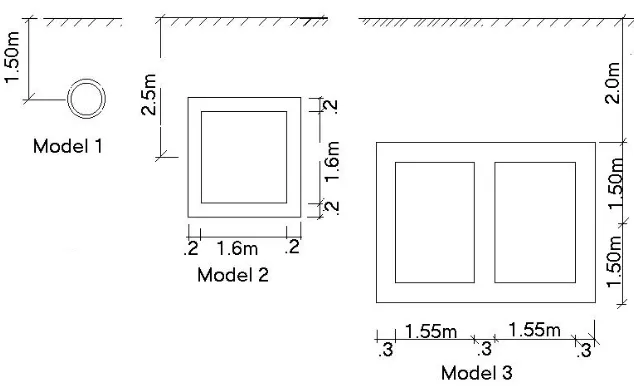
Description of the Structures
Fig. 1. Cross-sections of the 3 Models
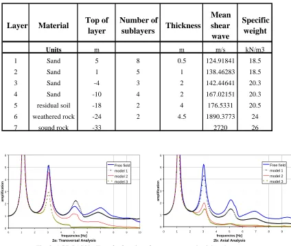
Soil profile
A horizontally layered sand deposit covering a residual soil is considered in the analyses. The sound rock is considered at a depth of -33m and the free surface is at an elevation of +5m. Table 2 presents the characteristics of the layered soil profile. The dynamic soil properties are obtained using the computer program SHAKE [1], which considers the responses associated with vertical propagation of shear waves through the linear visco-elastic system of horizontal layers. The input motion is correspondent to a peak acceleration of 0.1g.
COMPARISON OF RESULTS
Table 1. Properties of the beam cross-sections for the 3 Models
Model 1 Model 2 Model 3
E
kN/m2 2.1E+08 3.0E+07 3.0E+07Area
m2 0.0177 1.44 4.56Inertia
m4 0.001093 0.787 8.14mass
ton/m 0.139 4.32 13.7R
m 0.375 1 2Lenght
m 60 60 60f1
Hz 1.3 2.3 4.2f2
Hz 3.5 6.4 11.5f3
Hz 6.8 12.5 22.6f4
Hz 11.4 20.6Table 2. Properties of the layered soil profile
Layer
Material
Top of
layer
Number of
sublayers
Thickness
Mean
shear
wave
Specific
weight
Units m m m/s kN/m3
1 Sand 5 8 0.5 124.91841 18.5
2 Sand 1 5 1 138.46283 18.5
3 Sand -4 3 2 142.44641 20.3
4 Sand -10 4 2 167.02151 20.3
5 residual soil -18 2 4 176.5331 20.5
6 weathered rock -24 2 4.5 1890.3773 24
7 sound rock -33 2720 26
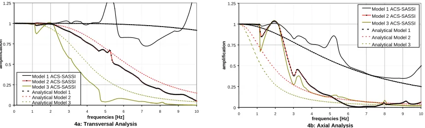
0 1 2 3 4 5 6
0 1 2 3 4 5 6 7 8 9 10
frequencies [Hz]
2a: Transversal Analysis
a
m
plif
ic
a
tion
Free field model 1 model 2 model 3
0 1 2 3 4 5 6
0 1 2 3 4 5 6 7 8 9 10
frequencies [Hz]
2b: Axial Analysis
a
m
plif
ic
a
tion
Free field model 1 model 2 model 3
0 0.2 0.4 0.6 0.8 1
0 1 2 3 4 5 6 7 8 9 10
frequencies [Hz]
3a: Transversal Analysis
a
m
plif
ic
a
tion
Model 1 Model 2 Model 3
0 0.2 0.4 0.6 0.8 1
0 1 2 3 4 5 6 7 8 9 10
frequencies [Hz]
3b: Axial Analysis
a
m
plif
ic
a
tion
Model 1 Model 2 Model 3
Fig. 3. Analytical transfer functions for transverse and axial analyses
By the analysis of the previous figures it can be noticed that, for flexible structures submitted to lower frequencies, the dynamical behavior is commanded by the soil. Structures with higher stiffness tend to have their correspondent transfer functions with lower responses for the same frequency excitations.
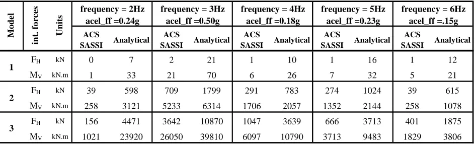
Fig. 4 present the comparison of the transfer functions from the analytical method with the relation between the transfer functions of each model to that obtained for the free-field from the ACS-SASSI. A relative good agreement for both axial and transversal analyses can be observed.
0 0.25 0.5 0.75 1 1.25
0 1 2 3 4 5 6 7 8 9 10
frequencies [Hz]
4a: Transversal Analysis
a
m
plif
ic
a
tion
Model 1 ACS-SASSI Model 2 ACS-SASSI Model 3 ACS-SASSI Analytical Model 1 Analytical Model 2 Analytical Model 3
0 0.25 0.5 0.75 1 1.25
0 1 2 3 4 5 6 7 8 9 10
frequencies [Hz]
4b: Axial Analysis
a
m
plific
a
tion
Model 1 ACS-SASSI Model 2 ACS-SASSI Model 3 ACS-SASSI Analytical Model 1 Analytical Model 2 Analytical Model 3
Fig. 4. ACS-SASSI relation between transfer functions: free-field / center of the model
Higher influence of soil-structure interaction effects for excitations close to the natural frequencies of the beam structures can be noticed. For example, the peaks at 6.8 and 11 Hz for Model 1, where the responses obtained from the ACS-SASSI are higher than those from the analytical solution. These effects, as well as the different seismic wave fields involved, can only be well evaluated and taken into account with the ACS-SASSI solution.
Tables 3 and 4 present some numerical values for internal forces obtained from the two methods for transversal and axial analyses. These results were obtained for 5 harmonic excitations at the control point for different frequencies. For the analytical solution the correspondent acceleration at the center of structure is used.
Coupling effects between vertical and axial responses in the ACS-SASSI method can be noticed. It is excited by the P / SV wave field which is correlated to circular motions of the soil particle during the seismic excitation.
CONCLUSIONS
Table 3. Internal forces obtained from the axial analysis
ACS
SASSI Analytical ACS
SASSI Analytical ACS
SASSI Analytical ACS
SASSI Analytical ACS
SASSI Analytical
N kN 210 2433 3957 3172 927 716 720 623 406 269
FV kN 0 0 0 0 0 0 0 0 0 0
MH kN.m 0 0 0 0 0 0 3 0 0 0
N kN 1277 12880 10830 15420 4206 3031 1335 2131 1317 671
FV kN 0 0 94 0 3 0 47 0 5 0
MH kN.m 4 0 660 0 28 0 230 0 27 0
N kN 1209 19760 7409 24700 3858 5146 966 3878 1087 1308
FV kN 2 0 107 0 29 0 74 0 18 0
MH kN.m 30 0 815 0 224 0 210 0 142 0
frequency = 5Hz acel_ff =0.23g
frequency = 6Hz acel_ff =.15g frequency = 2Hz
acel_ff =0.24g
frequency = 3Hz acel_ff =0.50g
frequency = 4Hz acel_ff =0.18g
Units
in
t. forces
Mod
el
1
2
3
TABLE 4: Internal forces obtained from the transversal analysis
ACS
SASSI Analytical ACS
SASSI Analytical ACS
SASSI Analytical ACS
SASSI Analytical ACS
SASSI Analytical
FH kN 0 7 2 21 1 10 1 16 1 12
MV kN.m 1 33 21 70 6 26 7 32 5 21
FH kN 39 598 709 1799 291 783 274 1024 39 615
MV kN.m 258 3121 5233 6314 1706 2057 1352 2144 258 1078
FH kN 156 4471 3642 10870 1047 3639 666 3713 401 1875
MV kN.m 1021 23920 26050 39810 6097 10790 3713 9483 1829 3806
frequency = 5Hz acel_ff =0.23g
frequency = 6Hz acel_ff =.15g frequency = 2Hz
acel_ff =0.24g
frequency = 3Hz acel_ff =0.50g
frequency = 4Hz acel_ff =0.18g
1
2
3
Mode
l
in
t. forces Units
REFERENCES
1.
"Shake – A Computer Program for Earthquake Response Analysis of Horizontally Layered Sites", Theoretical Manual– Version 1/1996 – University of California – Berkeley.
2.
A. Hindy and M. Novak: “Earthquake Response of Underground Pipelines”, Earthquake Engineering and StructuralDynamics -Vol.7 –1979.
3.
J.Lysmer; F. Ostadan; M. Tabatabaie; F. Tajirian ; S. Vahdani: “A System for Analysis of Soil-Structure Interaction” -SASSI2000 – User’s and Theoretical Manual – rev. 1 (1999) - Department of Civil and Environmental Engineering – University of California, Berkeley.