• No results found

Discriminating Between Weibull and Log-Logistic Distributions in Presence of Progressive Type II Censoring

N/A
N/A
Protected

Academic year: 2020

Share "Discriminating Between Weibull and Log-Logistic Distributions in Presence of Progressive Type II Censoring"

Copied!
10
0
0

Loading.... (view fulltext now)

Full text

(1)

Discriminating Between Weibull and

Log-Logistic Distributions in Presence of

Progressive Type II Censoring

Elsayed A. Elsherpieny

1

, Hiba Z. Muhammed

2

, Noha U. Radwan

3

1 Department of Mathematical Statistics, Institute of Statistical Studies and Research, Cairo University, Egypt 2Department of Mathematical Statistics, Institute of Statistical Studies and Research, Cairo University, Egypt,

3Ph.D.degrees from Institute of Statistical Studies and Research, Cairo University, Egypt

ABSTRACT: Weibull and log-logistic distributions are two popular distributions for analyzing lifetime data. In this paper, the problem of discriminating between these two distribution functions is considered in case of progressive type II censoring. Progressive type-II censored sampling is an important method of obtaining data in lifetime studies. Live units removed early on can be readily used in other tests, thereby saving cost to the experimenter, and a compromise can be achieved between time consumption and the observation of some extreme values. The ratio of the maximized likelihood test is used to discriminate between them. Some simulation experiments were performed to see how the probability of correct selection (PCS) under each model work for small sample sizes. Real data life is analyzed to see how the proposed method works in practice.

KEYWORDS: Weibull distribution; Log-logistic distribution; Progressive type-II censoring; Maximized likelihood ratio statistic; Probability of correct selection; Goodness of fit tests.

I. INTRODUCTION

Choosing the correct or best-fitting distribution for a given data set is an important issue. Most of the times distribution functions may provide a similar data fit but still it is desirable to select the correct or more nearly correct model and make the best possible decision based on observed data. Often choosing a particular model is difficult and the relevant effect of model miss selection can be quite severe.

The problem of choosing the correct model has been attempted by many researchers. Cox (1961) (see also Cox, 1962) was the pioneer in considering this problem. He also discussed the effect of choosing a wrong model. Since then extensive work has been done in discriminating between two or more distributions; see, e.g., Jackson (1968, Dumonceaux et al. (1973) , Dumonceaux and Antle (1973), Pereira (1977) , Bain and Engelhardt (1980) , Chen (1980), Kappenman (1982) , Firth (1988) , Pandey et al. (1991) , Fearn and Nebenzahl (1991) , Wiens (1999) Gupta and Kundu (2003,2004) , Pascual (2005) , Kundu and Manglick (2005) , Kundu and Raqab (2007) , Dey and Kundu (2009), Radwan (2009) , Dey and Kundu (2010) , Ashkar and Aucion (2012) , Raqab (2013) , Elsherpieny et al. (2013) and Rao and Kantam (2014) .

(2)

received signals level produced by some types of clutters, To model fading channels in wireless communications, In general insurance to model the size of reinsurance claims, and the cumulative development of asbestosis losses, In forecasting technological change In hydrology the Weibull distribution is applied to extreme events such as annual maximum one-day rainfalls and river discharges.

The log-logistic distribution (known as the Fisk distribution in economics) is a commonly used since the logarithm of the lifetime variables are logistically distributed and because of the well-known properties of this distribution and because it belongs to the location-scale family. It is used in lifetime data analysis It is used often as a parametric model for events whose rate increases initially and decreases later, for example mortality rate from cancer following diagnosis or treatment. It has also been used in hydrology to model stream flow and precipitation, and in economics as a simple model of the distribution of wealth or income. In networking The log-logistic has been used as a model for the period of time beginning when some data leaves a software user application in a computer and the response is received by the same application after travelling through and being processed by other computers (for example, when an application is displaying data coming from a remote sensor connected to the Internet). The log-logistic distribution provides one parametric model for survival analysis. Unlike the more commonly used Weibull distribution, it can have a non-monotonic hazard function: when shape parameter >1 the hazard function is unimodal (when shape parameter ≤ 1, the hazard decreases monotonically). The fact that the cumulative distribution function can be written in closed form is particularly useful for analysis of survival data with censoring.

In life testing and reliability studies, the experimenter may not always obtain complete information on failure times for all experimental units. Data obtained from such experiments are called censored data. Reducing the total test time and the associated cost is one of the major reasons for censoring. E.g., in medical or industrial applications, researchers have to treat the censored data because they usually do not have sufficient time to observe the lifetime of all subjects in the study. A censoring scheme, which can balance between (i) total time spent for the experiment; (ii) number of units used in the experiment; and (iii) the efficiency of statistical inference based on the results of the experiment, is desirable. The most common censoring schemes are Type-I (time) censoring, where the life testing experiment will be terminated at a prescribed time T, and Type-II (failure) censoring, where the life testing experiment will be terminated upon the r-th (r is pre-fixed) failure. Some procedures for selecting between distributions for the cases of not only complete but also censored samples for type- Ι censored and type –II censored samples , has been paid attention by some authors like: Siswadi and Quesenberry (1982), Kim et al. (2000) and Cain (2002). Block and Leemis (2008).Kim and Yum (2008 and Dey and Kundu (2012).

However, the conventional Type-I and Type-II censoring schemes do not have the flexibility of allowing removal of units at points other than the terminal point of the experiment. Because of this lack of flexibility, a more general censoring scheme called progressive Type-II right censoring has been introduced. As noted by Burkschat (2008), it is expected that a progressive censoring plan has longer test duration than a single (conventional Type-II) censoring plan in return for the gain in efficiency. Some of the earlier work on progressive censoring was conducted by Cohen (1963), Mann (1971) and Thomas and Wilson (1972). Several articles have been published on estimating the parameters of the unknown parameters for different distribution functions, see for example, Viveros and Balakrishnan (1991), Balakrishnan and Sandhu (1995), Balasooriya and Balakrishnan (2000), Balakrishnan and Kannan (2001), Balakrishnan et al. (2003, 2004), Mousa and Jaheen (2002). etc., a recent account on progressive censoring schemes can be obtained in the monograph by Balakrishnan and Aggarwala (2000) or in the excellent review article by Balakrishnan (2007). Progressive censoring schemes are very useful in life-test experiments and in clinical studies. Montanari and Cacciari (1988) reported results of progressively censored data aging tests on XLPE-insulated cable models under combined thermal-electrical stresses. Bhattacharya (2007) gives an example, in a clinical trial study. The monograph of Balakrishnan and Aggarwala (2000) and Balakrishnan (2007) gives an interesting review of the background and of developments in this field.

(3)

II. WEIBULL DISTRIBUTION

The p.d.f and c.d.fof Weibull denoted by WE(η,β), with scale parameter η > 0 and shape parameter β > 0 is given by:



x

e



x



x

we

f

(

;

,

)

1

,

,

>0

x

>0.

 

.

1

)

,

;

(

x

WE

x

e

F

Respectively, for 0 <β<1, the Weibull distribution has a decreasing hazard function. With β>1, the Weibull distribution has an increasing hazard function.For the special case when β= 1, the Weibull distribution is the simple exponential distribution.

If X has a Weibull distribution, then In(X) has an extreme value distribution. For β = 2, the Weibull distribution is the Rayleigh distribution. For a large value of the shape parameter, say β > 10.the shape of the Weibull distribution is close to that of the smallest extreme value distribution.

Also, for shape parameter values in the range 3<β<4, the shape of the Weibull distribution is close to that of the normal distribution. For much life data, the Weibull distribution is more suitable than the exponential, normal, and extreme value distributions.

Maximum likelihood function of Weibull distribution under progressive censoring

Let X1:m:n ,…, Xm:m:nbe progressively type II censored sample from a two parameter Weibull distribution, with

censoring scheme r= ( r1,…,rm ). The likelihood function is given by

i

r

n

m

i

x

F

m

i

i

m

n

x

f

k

we

L





 

)

:

:

(

1

1

)

:

:

(

)

,

(

Where

k

n

(

n

1

r

1

)

(

n

2

r

1

r

2

)...(

n

m

1

r

1

...

r

m1

).

For simplicity of notation, we will use

x

i instead of

x

i:m:n.

1

1

1

)

(

1

1

)

(

)

,

(

      

 





 

i

r

i m

i i m

i

x

e

x

m

k

i

r

i

x

F

m

i

x

f

k

we

L

The log likelihood function may then be written as,

 

,

1

)

1

(

1

ln

)

1

(

ln

ln

)

,

(

ln

i

x

m

i

i

r

m

i

i

x

m

m

we

L

(2.1)

Differentiating Equation (4.1) with respect to

and putting the derivative equal to zero we get

0

ˆ

1

)

1

(

)

1

`

ˆ

(

ˆ

ˆ

ˆ

ˆ

i

x

m

i

i

r

m

(4)

m i i i

x

r

m

1 ˆ ˆ

)

1

(

ˆ

 

(2.3)

 

ˆ 1 1 ˆ

)

)

1

(

(

ˆ

m i i i

x

r

m

. (2.4)

Differentiating Equation (2.1) with respect to

and putting the derivative equal to zero we get

   

 

ˆ

0

1

)

1

(

ˆ

ln

ˆ

ln

ˆ

1

)

1

(

ˆ

1

ln

ˆ

ln

ˆ

ˆ ˆ

 

i

x

m

i

i

r

i

x

i

x

m

i

i

r

m

i

i

x

m

m

(2.5)

 

ˆ

0

,

1

)

1

(

ˆ

ln

ln

ˆ

1

)

1

(

ˆ

1

ln

ˆ

ln

ˆ

ˆ ˆ

 

i

x

m

i

i

r

i

x

i

x

m

i

i

r

m

i

i

x

m

m

Byusing Equation (2.4) we get

   

,

0

1

)

1

(

ln

ˆ

1

)

1

(

1

ln

1

ˆ

1

ˆ

m

i

x

i

r

i

x

i

x

m

i

i

r

m

i

i

x

m

i

(2.6)

Therefore

ˆ

and

ˆ

can be obtained as a solutions of Equations (2.4) and (2.6).

III.LOG-LOGISTIC DISTRIBUTION

The p.d.f and c.d.f of log-logistic distribution denoted by LL(ε,σ), with scale parameter ε > 0 and shape parameter σ > 0 is given by:

,

2

)

/

(

1

1

)

/

)(

/

(

)

,

;

(





 

x

x

x

LL

f

,

> 0,

x

> 0.

.

)

/

(

1

)

/

(

)

,

;

(

x

x

x

F

LL

Maximum likelihood function of log-logistic distribution under progressive censoring

Let X1:m:n ,…, Xm:m:nbe progressively type II censored sample from a two parameter log-logistic distribution,

with censoring scheme r= ( r1,…,rm ). The likelihood function is given by

i

r

n

m

i

x

F

m

i

i

m

n

x

f

k

L

LL





 

)

:

:

(

1

1

)

:

:

(

)

,

(

Where

k

n

(

n

1

r

1

)

(

n

2

r

1

r

2

)...(

n

m

1

r

1

...

r

m1

).

(5)

ri i m i i m i m m LL

x

x

L

   

2 1 1 1

)

/

(

1

1

)

,

(

  

The logarithm of the likelihood function is given as

 

m i i i m i i

LL

m

m

x

r

x

L

1 1

)

/

(

1

ln

)

2

(

ln

)

1

(

ln

ln

)

,

(

ln

 . (3.1) Differentiating Equation (3.1) with respect to

and putting the derivative equal to zero we get:

0

ˆ

ˆ

)

ˆ

/

(

1

)

ˆ

/

(

)

2

(

ˆ

ˆ

1 ˆ ˆ

  m i i i i

x

x

r

m

L

(3.2)

.

)

ˆ

/

(

1

)

ˆ

/

(

)

2

(

1 ˆ ˆ

m i i i i

x

x

r

m

(3.3)

Differentiating Equation (3.1) with respect to

and putting the derivative equal to zero we get:

0

)

ˆ

/

(

1

)

ˆ

/

ln(

)

ˆ

/

(

)

2

(

ln

ˆ

ln

ˆ

1 ˆ

ˆ 1

  m i i i i i m i i

x

x

x

r

x

m

m

L

 

(3.4)

ln

ln

ˆ

0

)

ˆ

/

(

1

)

ˆ

/

(

)

2

(

ln

ˆ

ln

ˆ

1 ˆ

ˆ 1

 

  i m i i i i m i i

x

x

x

r

x

m

m

0

.

)

ˆ

/

(

1

ln

)

ˆ

/

(

)

2

(

ln

ˆ

1 ˆ

ˆ 1

  m i i i i i m i i

x

x

x

r

x

m

 

(3.5)

Therefore

ˆ

and

ˆ

can be obtained as a solutions of Equations (3.3) and (3.5).

IV.THE RATIO OF THE MAXIMIZED LIKELIHOOD (RML)

RML is defined as RML=

)

,

(

)

,

(

   

LL WE

L

L

.

Here

(

,

)

 

and

(

,

)

 

are the maximum likelihood estimators of

(

,

)

and

(

,

)

respectively. The test statistic T is the logarithm of RML and can be obtained as follows

)

,

(

ln

)

,

(

ln

)

,

(

)

,

(

ln

ln

       

LL WE LL WE

L

L

L

L

RML

T

In this discrimination procedure, choose: Weibull distribution if T > 0, i.e., if

ln

(

,

)

 

WE

L

>

ln

(

,

)

 

LL

(6)

The test statistic T can be used to compute the probability of correct selection (PCS) depends on the parent distribution, i.e., on the original distribution of the data x1,…,xn.That is, if the data are originally coming from Weibull distribution

the probability of correct selection (PCSWE) is given as

PCSWE = P (T > 0 | data follow Weibull distribution).

Also, if the data are originally coming from log-logistic distribution the probability of correct selection (PCSLL) is given

as

PCSLL = P (T < 0 | data follow log-logistic distribution).

V. NUMERICAL RESULTS

In this Section, the RML procedures are using for selecting between the Weibull and log-logistic distributions in presence of progressive type II censoring.

When the sample size is not sufficiently large, the PCS’s involved in the discrimination between the Weibull and the log-logistic distributions based on likelihood ratio can be determined with more accuracy through MC simulations sample. In this experiment generated progressively Type-II right censored order statistics from Weibull distribution or log-logistic distribution and calculated T then computed probability of correct selection ( PC). Monte Carlo runs are simulated based on different scheme given in Table 1.

i. First when the true distribution is Weibull distribution computation of the PCS is performed as follows:

By using the algorithm given by Balakrishna and Aggarwala (2000). The following steps are used to generate progressively Type-II right censored order statistics from Weibull distribution.

(1) Generate m independent uniform U(0,1), random variables W1, W2, ...,Wm.

(2) For given values of the progressive censoring scheme R1, R2, ..., Rm. set

m

i

W

V

m i m j

j

R i i

i 1

,

1

,

2

,...,

/

1



  

   

  

(3) Set Ui = 1−VmVm−1...Vm−i+1 for i = 1,2,..., m. Then U1:m:n, U2:m:n,....,Um:m:nis a progressively Type-II right censored

sample of size m from U(0,1).

(4) For a given values of the two parameters η and β

m

i

u

X

i

ln(

1

)

,

1

,

2

,...,

/ 1

is a progressively Type-II right censored sample of size m from the Weibull distribution. We generate a progressively Type-II right censored samples from the Weibull distribution at η=1 andβ = 0.5, 1, 1.5, 2, 2.5, 3, 5. (5) By maximum likelihood, both the weibull and the log-logistic distributions are fitted to the sample (x1, x2, · · · , xm),

and a realization, t, of the statistic

LL we

L

L

T

ln

, is calculated and stored.

(6)Steps 4 and 5 are repeated many times (in this study, the repetition was done 100 times). (7) The approximate PCS under the assumption that the true distribution is weibull is:

PCSwe=Pr[ T>0]≈ (number of t values in step 5 > 0)/100 .

The result are given in Table (2).

ii. Second when the true distribution is log-logistic distribution computation of the PCS is performed as follows:

The same steps in (1) , (2) , (3) are used.

(4) For a given values of the two parameters ε and σ

m

i

u

u

X

i

,

1

,

2

,...,

1

/ 1

(7)

is a progressively Type-II right censored sample of size m from the log-logistic distribution.We generate a progressively Type-II right censored samples from the log-logistic distribution at ε =1 and σ = 0.5, 1, 2, 4, 8.

(5) By maximum likelihood, both the weibull and the log-logistic distributions are fitted to the sample(x1, x2, · · · , xm),

and a realization, t, of the statistic

LL we

L

L

T

ln

, is calculated and stored.

(6) Steps 4 and 5 are repeated many times (in this study, the repetition was done 100 times).

(7) The approximate PCS under the assumption that the true distribution is log-logistic is: PCSLL=Pr[ T<0]≈ (number

of t values in step 5 < 0)/100 .

The result is given in Table (3).

Table 1. Different schemes of progressively censored Schemes n M censoring scheme (R) I 10 4 [2 0 2 2]

II 15 6 [2 0 2 0 3 2] III 20 8 [1 2 0 2 3 2 0 2] IV 25 10 [4 0 0 2 0 0 4 2 0 3]

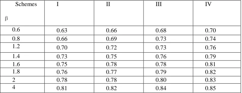
Table 2. The probability of correct selection (PCS) based on Monte Carlo simulations (MC) when the data are from Weibull distribution

IV III

II I

Schemes

β

0.70 0.68

0.66 0.63

0.6

0.74 0.73

0.69 0.66

0.8

0.76 0.73

0.72 0.70

1.2

0.79 0.76

0.75 0.73

1.4

0.81 0.78

0.78 0.75

1.6

0.82 0.79

0.77 0.76

1.8

0.83 0.80

0.78 0.78

2

0.85 0.84

0.82 0.81

4

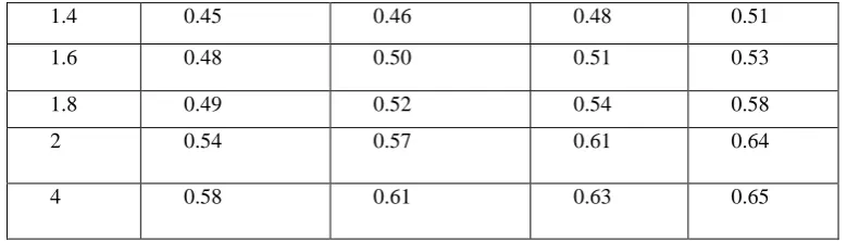
Table 3. The probability of correct selection (PCS) based on Monte Carlo simulations (MC) when the data are from log-logistic distribution

IV III

II I

Schemes σ

0.44 0.42

0.41 0.38

0.6

0.43 0.41

0.40 0.39

0.8

0.47 0.46

0.46 0.44

(8)

0.51 0.48

0.46 0.45

1.4

0.53 0.51

0.50 0.48

1.6

0.58 0.54

0.52 0.49

1.8

0.64 0.61

0.57 0.54

2

0.65 0.63

0.61 0.58

4

Noticed that the PCS works quite well even for small sample sizes. Interestingly, It is quite clear from Tables 2 and 3 that as the sample size increases the PCS increases as expected. It is also clear that as the shape parameter moves away from 1, the PCS increases. whenWeibull is the true distribution, then the PCS based on Monte Carlo simulation is found to be significantly higher than the other case particularly for small sample sizes. For example, for scheme 1 when the sample size is 20, m=8 , and the true distribution is Weibull, the PCS is 0.63. But when the true distribution is log-logistic, for the same sample size the PCS is only 0.38.

VI.DATA ANALYSIS

To illustrate the use of the estimation methods proposed in this thesis, the following example is discussed.

Example. Nelson [1982, p.228, table 6.1] presented data on the time to breakdown of an insulating fluid in an accelerated test at 34 kilovolts. This data is given in Table 4.

Table 4. Nelson's Data

0.19 0.78 0.96 1.31 2.78 3.16 4.15 4.67 4.85 6.50 7.35 8.01 8.27 12.06 31.75 32.52 33.91 36.71 72.89

For the purposes progressively type II censored sample of size m=8 was randomly selected from the n=19 observations, as given by Viveros and Balakrishman (1994). The observations and censoring scheme are reported in Table5.

Table 5. Progressively type II censored sample generated from the times to breakdown data

I 1 2 3 4 5 6 7 8 xi 0.19 0.78 0.96 1.31 2.78 4.85 6.50 7.35

Ln xi -1.660 -0.248 -0.040 0.270 1.022 1.578 1.871 1.994

ri 0 0 3 0 3 0 0 5

From the formula described in Section (2) and section (3), we obtain the MLEs of η , β to be

ˆ

= 0.576 and

ˆ

= 0.42 for the Weibull distribution , then ln L

WE = -35.7752 , and we obtain the MLEs of

and

to be

ˆ

=

0.9027 and

ˆ

= 1.233 for the log-logistic distribution, then ln LLL = -39.3475

Now using the following formula derived in Section (3.1) we calculate T.

)

,

(

ln

)

,

(

ln

)

,

(

)

,

(

ln

ln

  

 

  

LL WE

LL

WE

L

L

L

L

RML

T

(9)

Therefore, by using the maximum likelihood ratio test to discriminate between Weibull and log-logistic distributions in case of progressive censoring Type II censored sample, the Weibull model is chosen for this data set.

VII. CONCLUSION

Weibull and log-logistic distributions are two popular distributions for analysing lifetime data. In this thesis, the problem of discriminating between these two distribution functions is considered in case of censored samples. A censoring scheme called progressive type II censoring is considered. A hypothesis testing method is used in which it is assumed that a data are coming either from Weibull or log-logistic distribution. Then the ratio of the maximized likelihood test is used to discriminate between them. Some simulation experiments were performed to see how the probability of correct selection (PCS) under each model work for small sample sizes. We observed that the PCS works quite well even for small sample sizes. It is quite clear that as the sample size increases the PCS increases as expected. It is also clear that as the shape parameter moves away from 1, the PCS increases. Interestingly, when Weibull is the true distribution, then the PCS based on Monte Carlo simulation is found to be significantly higher than the other case particularly for small sample sizes. Real data life is analysed to see how the proposed method works in practice.

REFERENCES

[1] Aucoin, F., and Ashkar ,F., (2012). Choice between competitive pairs of frequency models for use in hydrology: a review and some new results. Hydrological Sciences Journal, vol. 57, no.6, 1092–1106.

[2] Bain, L. J., and Engelhardt, M., (1980). Probability of correct selection ofWeibull versus gamma based on likelihood ratio.

Communicationsin Statistics, Theory and Methods, vol. 9, no.6, 375-381.

[3] Balasooriya, U. and Balakrishnan, N. (2000), “Reliability sampling plan for log-normal distribution”, IEEE Transactions on Reliability, vol. 49, 199 – 203.

[4] Balakrishnan, N. and Aggarwala, R. (2000). Progressive censoring: theory, methods and applications. Birkhauser, Boston.

[5] Balakrishnan, N. and Kannan, N. (2001), “Point and interval estimation for parameters of the logistic distribution based on progressively type-II censored data”, Handbook of Statistics, vol. 20, North Holland, Amsterdam.

[6] Balakrishnan, N., Kannan, N., Lin, C.T. and Ng, H. (2003). Point and interval estimation for Gaussian distribution based on progressively Type-II censored samples. IEEE Trans. Reliab., 52, 90-95.

[7] Balakrishnan, N., Kannan, N., Lin, C.T. and Wu, S.J.S. (2004), “Inference for the extreme value distribution under progressive type-II censoring”, Journal of Statistical Computations and Simulations, 25 - 45.

[8] Balakrishnan, N. and Sandhu, R.A. (1995), “A simple algorithm for generating progressively type-II generated samples”, American Statistician, vol. 49, 229 - 230.

[9] Balakrishnan, N. (2007), “Progressive Censoring Methodology: An Appraisal”, (with discussions), TEST, vol. 16, no. 2, 211 – 296. [10] Bhattacharya, B. (2007). Testing for ordered failure rates under general progressive censoring. J.Statist. Plann. Inference 1 37, 1775_1786. [11] Block, A.D., Leemis, L.M., (2008). Parametric model discrimination for heavily censored survival data. IEEE Transactions on Reliability,

vol.57, no.2, 248-259.

[12] Burkschat, M., On optimality of extremal schemes in progressive Type II censoring. Journal of Statistical Planning and Inference 138 (2008), 1647–1659.

[13] Cain, S.R., (2002). Distinguishing between lognormal and Weibull distributions. IEEE Transactions on Reliability, vol.51, no.1, 32-38. [14] Chen, W. W. (1980). On the tests of separate families of hypotheses with small sample size. Journal of Statistical Computations and

Simulations, vol. 2, 183-187.

[15] Cohen, A.C. (1966), “Life testing and early failure”, Technometrics, vol. 8, 539 - 549.

[16] Cox, D. R. (1961). tests of separate families of hypotheses. Proceeding of the Fourth Berkely Symposium in Mathematical Statistics and Probability, Berkely, University of California Press, pp. 105-123.

[17] Cox, D. R. (1962). Further results on tests of separate families of hypo-theses. Journal of the Royal Statistical Society, Series B, vol. 24, 406-424.

[18] Dey, A. K., and Kundu, D. K. (2009). Discriminating among the log-normal, Weibull and generalized exponential distributions. IEEE Transactions on Reliability , vol. 58, no. 3, 416-424.

[19] Dey, A. K., and Kundu, D. K. (2010). Discriminating between the log-normal and log-logistic distributions. Communications in Statistics, Theory and Methods, vol. 39, 280 – 292.

[20] Dey, A. K., and Kundu, D. K. (2012). Discriminating between the Weibull and Log-normal distributions for type-II censored data.

Statistics ,vol. 46, no. 2, 197 - 214.

[21] Dumonceaux, R., and Antle., C.E. (1973). Discriminating between the log-normal and Weibull distribution. Technometrics, vol. 15, no.4, 923-926.

[22] Dumonceaux, R., Antle, C., and Hass, G. (1973). Liklihood ratio test for discrimination between two models with unknown location and scale parameters. Technometrics, 19-27.

(10)

[24] Fearn, D. H., and Nebenzahl, E. (1991). On the maximum likelihood ratio method of deciding between the Weibull and gamma dist ributions.

Communications in Statistics, Theory and Methods, vol. 20, 579-593.

[25] Firth, D. (1988). Multiplicative errors: log-normal or gamma?. Journal of the Royal Statistical Society, Series B, no.2, 266-268.

[26] Gupta, R. D., and Kundu, D. k. (2003). Discriminating between Weibull and generalized exponential distributions. Journal of Computational Statistics and Data Analysis, vol.43, 179 – 196.

[27] Gupta, R. D., and Kundu, D. k. (2004). Discriminating between the gamma and generalized exponential distributions. Journal of Statistical Computation and Simulation, vol. 74, no.2, 107-121.

[28] Jackson, O. A. Y. (1968). Some results on tests separate families of hypo- theses. Biometrika, vol. 55, 355-363.

[29] Kappenman, R. F. (1982). On a method for selecting a distributional model. Communication in Statistics, Theory and Methods, vol.11, 663-672.

[30] Kim, D.H., Lee, W.D., Kang, S.G., (2000). Bayesian model selection for life time data under type II censoring. Communications in Statistics-Theory and Methods, vol.29, no.12, 2865-2878.

[31] Kim, J.S. and Yum, B-J., (2008). Selection between Weibull and log-normal distributions: A comparative simulation study. Computational Statistics and DataAnalysis, vol. 53, 477 - 485.

[32] Kundu, D. K., and Manglick, A. (2004). Discriminating between Weibull and log-normal distributions. Naval Research Logistics (NRL),vol. 51, Issue 6, 893–905.

[33] Kundu, D. K., and Manglick, A. (2005). Discriminating between the log-normal and gamma distributions. Journal of the Applied Statistical Sciences, vol.14, 175-187.

[34] Kundu, D., Raqab, M. Z. (2007). Discriminating Between the Generalized Rayleigh and Log-Normal Distribution. Statistics, vol.41 no.6, 505-515.

[35] Mann, N.R. (1971), “Best linear invariant estimation for Weibull parameters under progressive censoring”, Technometrics, vol. 13, 521 - 533.

[36] Montanari, G.C. and Cacciari, M. (1988). Progressively-censored aging tests on XLPE-insulated cable models. IEEE Trans. Electrical Insul. 23 , 365_372.

[37] Mousa, M. and Jaheen, Z. (2002). Statistical inference for the Burr model based

[38] on progressively censored data. An international Computers &Mathematics with

[39] applications, 43, 1441-1449.

[40] Pascual, F. G. (2005). Maximum likelihood estimation under misspecified log-normal and Weibull distributions. Communications in Statistics, Simulation and Computations, vol. 34, 503-524.

[41] Pandey, M., Ferdous, J. and Uddin, M. B. (1991). Selection of probability distributions for life testing data. commun. Statist.-Theory Meth., 20(4), 1373-1388.

[42] Pereira, B. de B. (1977). A note on the consistency and on the finite sample comparisons of some tests of separate families of hypotheses.

Biometrika, vol. 64, 109-113.

[43] Radwan. AL-E. B.(2009). On the distribution of the ratio of the maximized likelihoods (RML) statistic. M.Sc in statistic. ISSR.

[44] Raqab, M. Z. (2013). Discriminating between the generalized Rayleigh and Weibull distributions. Journal of Applied Statistics, vol. 40, no.7, 1480-1493.

[45] Rao, S. B. and Kantam L. R. R. (2014). Discriminating between log-logistic and rayleigh distributions, Pak.j.stat.oper.res., Vol.X, no.1,1-7.

[46] Siswadi, Quesenberry, C.P., (1982). Selecting among Weibull, lognormal and gamma distributions using complete and censored sa mples.

Naval Research Logistics Quarterly 29. no.4, 557-569.

[47] Thomas, D.R. and Wilson, W.M. (1972), “Linear order statistic estimation for the twoparameterWeibull and extreme value distributions from type-II progressively censored samples”, Technometrics, vol. 14, 679 - 691.

Figure

Table 2. The probability of correct selection (PCS) based on Monte Carlo simulations (MC) when the data are from Weibull distribution
Table 5. Progressively type II censored sample generated from the times to breakdown data  I 1 2 3 4 5 6

References

Related documents