Surface Earthquake Fault Simulation Using High Performance Computing for Consideration of Uncertainty

Transactions, SMiRT-25 Charlotte, NC, USA, August 4-9, 2019

Division III

SURFACE EARTHQUAKE FAULT SIMULATION USING HIGH

PERFORMANCE COMPUTING FOR CONSIDERATION ON

UNCERTAINTY

Kazumoto Haba

, Masataka Sawada

, and Muneo Hori

1_{Manager, Taisei Corporation, Shinjuku-ku, Tokyo, Japan ([email protected])}

2_{Research Engineer, Nuclear Risk Research Center, Central Research Institute of Electric Power Industry,}

Abiko, Chiba, Japan

3_{Principal Scientist, Japan Agency for Marine-Earth Science and Technology, Yokohama, Kanagawa,}

Tokyo, Japan

INTRODUCTION

Surface fault displacements can cause extensive damage to infrastructure and buildings, and therefore, reliable estimations of surface fault displacements become necessary for safety of nuclear power plants (NPPs). In this regard, numerical simulations of fault rupture processes are a candidate for the estimation of fault displacement. We have developed a high-performance computing finite element method (HPC-FEM) (Sawada et al. (2017)) based on the FrontISTR (FrontISTR Forum (2018)) for the simulation and applied HPC-FEM to simulate an actual earthquake (Sawada et al. (2018)). For a reliable estimation, it is essential to consider various uncertainties in the fault rapture process, such as those of the initial stress distribution, material properties, and asperity on the primary fault plane, etc. Here, we evaluate the effects of these uncertainties by capacity computing with the proposed HPC-FEM.

SIMULATION CONDITIONS

Simulation Method

It is improbable that NPPs can be located above the primary fault on the surface, as detailed geological surveys are conducted explicitly to eliminate this possibility. Therefore, the purpose of fault displacement evaluation for NPPs is to estimate the possibility of the occurrence of secondary fault displacement accompanying the primary fault activity. The following two-step simulation is reasonable for this aim: 1) evaluation based on the elastic theory of dislocations (Okada (1985)) of the crustal deformation caused by the primary fault slip.; and 2) evaluation of the displacement and deformation of the target area around NPPs by analyzing a detailed 3D model with HPC-FEM, wherein the displacement calculated in step 1) is applied to the boundary of the target area. In these simulations, it is important to estimate the critical base slip ΔC that makes the rupture reach the ground surface. The probability of surface fault displacement can be quantified by ΔC based on the same treatment of the earthquake PRA because the primary fault slip is associated with the earthquake magnitude. For practical reasons, the multiple quasi-static simulation is used to evaluate the effect of uncertainties.

Simulation Condition of Standard Case

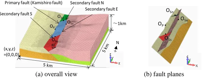
and three secondary faults based on observational results (see Table 1). Position at y =3.85 km on the surface of the primary fault in the analytical model corresponds to the north end of the observed surface fault displacement in Figure 1. The number of geological layers is set to two based on elastic wave velocity, which was acquired from the subsurface structure database of the Japan Seismic Hazard Information Station (NIED (2019)). In the model, the rock mass and fault planes are modeled by the use of second-order tetrahedral elements and second-order triangle joint elements, respectively. This model has 2.17 million degrees of freedom.

Figure 1. Surface fault displacement distribution based on differential analysis of multiple LiDAR-DEM datasets (Aoyagi (2016)).

(a) overall view (b) fault planes

Figure 2. Standard analytical model with ~2.7 million degrees of freedom. The model has two geological layers and four fault planes, which are indicated by boundaries of the colored blocks. The points OP, OSe,

OSs and OSn denote the evaluation point of the fault planes on the surface in this simulation.

Table 1: Configuration of fault planes in standard analytical model

Fault Strike Dip Position relative to primary fault

Primary fault (Kamishiro fault)

North-northeast

(+y-direction) 40° -

Secondary fault E South-southwest 40° 0.5 km east from primary fault

Secondary fault N East-northeast 40° Connected to primary fault

at y = 3.85 km and the surface of the ground

Secondary fault S West-southwest 40° Connected to primary fault at y = 1.35 km and ground surface

We use a nonlinear spring model as a constitutive law to represent the fault slip. The spring coefficient per unit area (shear stiffness) k is described by the following function of slip u:

𝑘 = {

𝑘

− (𝑘

− 𝑘

)𝑢/𝑢

(𝑢 ≤ 𝑢

)

𝑘

(𝑢

≤ 𝑢)

,

(1)

Secondary fault N

Secondary fault E

Secondary fault S

Primary fault (Kamishiro fault)

～1km

(x,y,z) =(0,0,0)

N 40°

Primary fault (Kamishiro fault)

Secondary fault S

Secondary fault N Secondary fault E

OP

OSs

OSe

OSn

OP

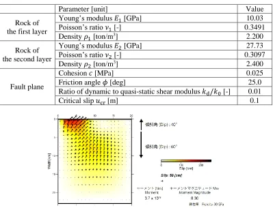
where 𝑘0 denotes the quasi-static shear stiffness (initial shear stiffness), 𝑘d denotes the dynamic shear stiffness (final shear stiffness), and 𝑢cr denotes the critical slip (see Figure 3 a)). The slip–traction relationship (Figure 3 b)) exhibits a peak strength 𝜏max. Further, slip u can rapidly increase when the external force becomes larger than 𝜏max. The peak strength 𝜏max depend on normal stress as the following relationship: 𝜏max = 𝜎𝑛tan 𝜙 + 𝑐. Here, 𝑐 and 𝜙 denote the cohesion and friction angle, respectively, and

𝜎𝑛 denotes the normal stress on the fault plane. Table 2 lists the material properties in the standard case, which are the same as the ones used by Sawada et al. (2018)

The slip distribution across the Kamishiro fault, which corresponds to the initial condition of the elastic theory of dislocations, was set based on the result of source inversion obtained from the Geospatial Information Authority of Japan (2014) (see Figure 4).

a) slip–spring coefficient relationship b) slip–traction relationship

Figure 3. Constitutive law for fault plane

Table 2: Material properties for standard case

Parameter [unit] Value

Rock of the first layer

Young’s modulus 𝐸1 [GPa] 10.03

Poisson’s ratio 𝜈1 [-] 0.3491

Density 𝜌1 [ton/m3] 2.200

Rock of the second layer

Young’s modulus 𝐸2 [GPa] 27.73

Poisson’s ratio 𝜈2 [-] 0.3097

Density 𝜌2 [ton/m3] 2.400

Fault plane

Cohesion 𝑐 [MPa] 0.025

Friction angle 𝜙 [deg] 25.0

Ratio of dynamic to quasi-static shear modulus 𝑘d/𝑘0 [-] 0.01

Critical slip 𝑢cr[m] 0.1

Figure 4. Slip distribution on Kamishiro fault as obtained by source inversion (GIAJ (2014)) 0.0

5.0 10.0 15.0 20.0

0.00 0.05 0.10 0.15 0.20 0.25 0.30

k

/

σn

[1

/m

]

Slip u[m]

0.00 0.10 0.20 0.30 0.40 0.50

0.00 0.05 0.10 0.15 0.20 0.25 0.30

τ

/

σn

[-]

Slip u[m]

Multiple simulations were conducted considering the uncertainties of material properties, slip distributions on the primary fault, analytical models.

UNCERTAINTY IN FAULT DISPLACEMENT SIMULATION

In this section, we explain the uncertainties of the input conditions in our fault displacement simulations. Uncertainty can be classified as aleatory and epistemic uncertainty.

Epistemic uncertainty refers to the scientific uncertainty in the model of the process, which is due to limited data and knowledge. In the simulation in which fault planes are set as known weak planes, the epistemic uncertainty includes the uncertainties of the strikes and dips of the fault planes and slip distribution across the primary fault plane and its slip value. Because the slip value of the primary fault is associated with the seismic moment, the slip uncertainty corresponds to the uncertainty of the earthquake magnitude. It is to be noted that the uncertainty of the slip value of the primary fault can be evaluated by means of a one-time quasi static simulation in which the slip is incrementally loaded on the boundary of the analytical model. For other epistemic uncertainties, the uncertainty of response must be evaluated by use of alternative models and parameter values with, for e.g., logic trees.

Aleatory uncertainty refers to the natural randomness in a process. In fault displacement simulations, the uncertainties of the material properties of rocks and fault planes correspond to aleatory uncertainty. For continuous variables with a probability density function, the uncertainty of response can be evaluated via repetitive simulations with, for e.g., the Monte Carlo method.

In this study, we consider the uncertainties of slip distribution across the primary fault, configuration of secondary fault E, and material properties.

Uncertainty of Slip Distribution across Primary Fault

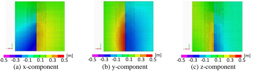
Figure 5 shows the input displacement on the bottom boundary of the analytical model obtained by the elastic theory of dislocations with the use of source inversion (GIAJ (2014)). We also consider the slip distribution wherein superficial part which is shallower than E.L. -3 km is corrected by use of the observed surface slip distribution (see Figure 6). Furthermore, we consider slip distribution in which the surface slip does not appear in the northern side of y = 3.85 km which corresponds to the north end of the observed surface fault displacement in Figure 1. The condition can be realized by increasing the quasi-static shear modulus 𝑘0 in the superficial part within E.L. ~0.25 km at y > 3.85 km.

(a) x-component (b) y-component (c) z-component

Figure 5. Input displacement on bottom boundary of model (GIAJ (2014) distribution)

(a) x-component (b) y-component (c) z-component

Figure 6. Input displacement on bottom boundary of model (corrected distribution)

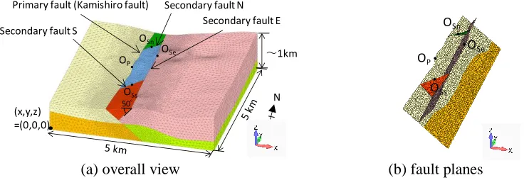
Uncertainty of Configuration of Secondary Fault

We consider the case with dip angle = 50° of secondary fault E in addition to the dip angle 40°

(standard case). Figure 7 shows the analytical model with dip angle = 50° of secondary fault E.

(a) overall view (b) fault planes

Figure 7. Analytical model with dip angle = 50° of secondary fault E. Other conditions are the same as ones of the standard analytical model in Figure 2

Material Properties

The Young’s modulus of the rocks and the friction angle of the fault planes are assumed to be log-normal random variables, in which the Young’s modulus and friction angle have coefficients of variance (COVs) of 30% and 15%, respectively. In the study, we conducted parametric studies using the cohesion,

ratio of dynamic to quasi-static shear modulus, and

Table 3

Table 3: Material properties utilized for parametric studies. The values indicated in boldface correspond to the standard-case values listed in Table 2.

Parameter [unit] value 1 value 2 value 3

Young’s modulus [GPa] first layer 𝐸1 7.21 10.03 13.39

second layer 𝐸2 19.41 27.73 36.05

Friction angle 𝜙 [deg] 21.25 25.0 28.75

Cohesion 𝑐 [MPa] 0.000 0.025 -

Ratio of dynamic to quasi-static shear modulus 𝑘d/𝑘0 [-] 1/1000 1/100 1/20

Critical slip 𝑢cr[m] 0.10 0.60 1.5

-0.5 -0.3 -0.1 0.1 0.3 0.5[m] -0.5 -0.3 -0.1 0.1 0.3 0.5[m] -0.5 -0.3 -0.1 0.1 0.3 0.5[m]

Primary fault (Kamishiro fault)

～1km Secondary fault S

Secondary fault N Secondary fault E

(x,y,z) =(0,0,0)

N 50°

OP

OSs

OSe

OSn

OP

RESULTS

Standard Case with Corrected Distribution

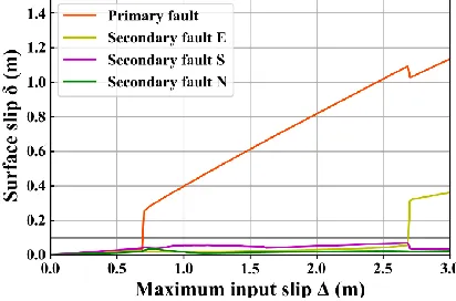
We first examine the standard-case results with the corrected slip distribution on the primary fault. Figure 8 and Figure 9 show the contours of the slip distribution on the fault planes at Δ = 1.5 m and 2.8 m, respectively. The input base slip propagates and disperses on the primary fault, and the slip reaches the ground surface. Although the slip on any secondary faults does not appear at Δ = 1.5 m, the surface slip appears on secondary fault E at Δ = 2.8 m. Under this condition, the slip does not appear on secondary faults S and N.

Figure 10 shows the relationship between the maximum input slip at the bottom of the model and surface slip at the observed surface points. Surface fault displacement occurs when the base slip of the primary fault becomes larger than a critical value, that is, the critical base slip ΔC. The ΔC values of the primary fault and secondary fault are 0.705 m and 2.700 m, respectively. Under this condition, the surface slip does not appear at the observed surface point of the secondary faults S and N.

(a) primary fault (b) secondary fault E (c) secondary faults S and N

Figure 8. Slip contour on fault planes at Δ = 1.5 m (case of corrected slip distribution)

(a) primary fault (b) secondary fault E (c) secondary faults S and N

Figure 9. Slip contour on fault planes at Δ = 2.8 m (case of corrected slip distribution)

Figure 10. Relationship between maximum input slip and surface slip at evaluation points (case of corrected slip distribution)

0.0 0.2 0.4 0.6 0.8 1.0[m] OP

0.0 0.2 0.4 0.6 0.8 1.0[m] OSe

0.0 0.2 0.4 0.6 0.8 1.0[m]

OSs _O

Sn

0.0 0.2 0.4 0.6 0.8 1.0[m] OP

0.0 0.2 0.4 0.6 0.8 1.0[m] OSe

0.0 0.2 0.4 0.6 0.8 1.0[m]

OSs _O

Uncertainty of Slip Distribution across Primary Fault

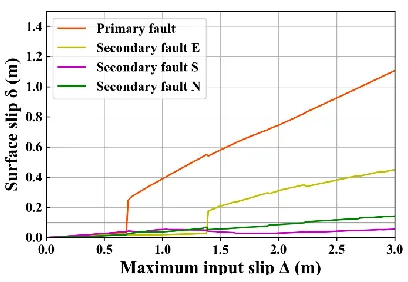
Figure 11 and Figure 12 show the contour of the slip distribution and the relationship between the maximum base slip and surface slip for the GIAJ (2014) slip distribution, respectively. These results indicate that the slip distribution on the primary fault is wider than the corrected slip distribution. In the case with the GIAJ (2014) slip distribution, the slips of secondary faults E and N do not appear, but that of the secondary fault S appears near the connection with the primary fault.

(a) primary fault (b) secondary fault E (c) secondary faults S and N

Figure 11. Contour of slip on fault planes at Δ = 2.8 m (case of GIAJ (2014) slip distribution）

Figure 12. Relationship between maximum input slip and surface slip at evaluation point (case of GIAJ (2014) slip distribution)

Figure 13 and Figure 14 show the contour of the slip distribution and relationship between the maximum base slip and surface slip, respectively, in the case of the corrected slip distribution with the slip fixed in the northern area. We find from Figure 13 that the slip in the superficial part within E.L. ~0.25 km in the northern portion at y > 3.85 km reduces to a small value. The slips of secondary faults E and N appear, but that of secondary fault S does not appear.

(a) primary fault (b) secondary fault E (c) secondary faults S and N

Figure 13. Contour of slip on fault planes at Δ = 2.8 m (case of corrected slip distribution with fixed slip in northern area）

0.0 0.2 0.4 0.6 0.8 1.0[m] OP

0.0 0.2 0.4 0.6 0.8 1.0[m] OSe

0.0 0.2 0.4 0.6 0.8 1.0[m]

OSs _O

Sn

0.0 0.2 0.4 0.6 0.8 1.0[m] OP

0.0 0.2 0.4 0.6 0.8 1.0[m] OSe

0.0 0.2 0.4 0.6 0.8 1.0[m]

OSs _O

Figure 14. Relationship between maximum input slip and surface slip at evaluation point (case of corrected slip distribution with fixed slip in northern area)

These results indicate that the occurrence of the secondary fault displacement strongly depends on the slip distribution on the primary.

Uncertainty of Configuration of Secondary Fault

We show the results in the case of the corrected slip distribution with dip angle = 50° of secondary fault E. The values of the critical base slip ΔC of the primary and secondary faults are 0.705 m and 2.595 m, respectively. Under this condition, the surface slip does not appear at the evaluation points of secondary faults S and N in common with the standard case with dip angle = 40° of secondary fault E. This result indicates that the ambiguity of the dip angle of the secondary fault have an insignificant effect on the occurrence of secondary fault displacement.

Material Properties

Figure 15 shows the histogram of the critical base slip ΔC in the case with uncertain Young’s modulus and friction angle; the histogram was obtained via 120 repetitive calculations with Latin hypercube sampling. The green line in Figure 15 indicates the fitting result of the log-normal distribution. This result indicates that the probabilistic distribution of ΔC can be approximated by the log-normal distribution. Subsequently, the mean and standard deviation of ΔC for the secondary fault E are found to be 2.71 m and 0.26 m, respectively.

(a) primary fault (b) secondary fault E

Figure 15. Probabilistic distribution of critical base slip ΔC. The histograms depict the results of 120 repetitive calculations. The green line denotes the fitting result of the log-normal distribution.

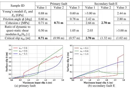
Table 4: Critical base slip, which is the maximum input slip when the surface slip equals 0.1 m for the first time, as obtained by parametric studies. The boldface values correspond to the results of the standard

case. Values 2 and 3 of critical slip in parentheses may correspond to dislocation.

Sample ID Primary fault Secondary fault E

Value 1 Value 2 Value 3 Value 1 Value 2 Value 3 Young’s moduli 𝐸1 and

𝐸2 [GPa] 0.88 m

0.71 m

0.60 m >3.00 m

2.70 m

2.44 m

Friction angle 𝜙 [deg] 0.60 m 0.78 m 2.42 m 2.80 m

Cohesion 𝑐 [MPa] 0.71 m - 2.66 m -

Ratio of dynamic to quasi-static shear modulus 𝑘d/𝑘0 [-]

0.50 m 1.05 m 2.03 >3.00 m

Critical slip 𝑢cr[m] 0.71 m (0.98 m) (0.57 m) 2.70 m (1.32 m) (1.02 m)

(a) primary fault (b) secondary fault E

Figure 16. Relationship between maximum input slip and surface slip at observed point (case of parameter study for critical slip)

CONCLUSION

In this study, we evaluated the effect of some uncertainties in the input condition via multiple HPC-FEM simulations. The uncertainty in fault displacement simulations can be classified as aleatory

0.0 1.0 2.0 3.0 4.0

0.0 0.5 1.0 1.5 2.0 2.5 3.0 3.5 P rob abi li sti c de ns ity [ -]

Critical base slip[m]

0.0 1.0 2.0 3.0 4.0

0.0 0.2 0.4 0.6 0.8 1.0 1.2 1.4 1.6 1.8 P rob abi li sti c de ns ity [ -]

and epistemic uncertainty. In the simulation in which fault planes are set as known weak planes, the epistemic uncertainty includes the uncertainties of the strikes and dips of fault planes and slip distribution across the primary fault plane and its slip value. Meanwhile, uncertainties of the material properties of rocks and fault planes correspond to aleatory uncertainty. In this study, we consider the uncertainties of slip distribution across the primary fault and the configuration of secondary fault E as the epistemic uncertainty and those of the material properties as the aleatory uncertainty. As a result, we find that the uncertainties of slip distribution across the primary fault strongly affect the occurrence of secondary fault displacement. The critical base slip depends on the uncertainties of the material properties. In particular, the critical base slip ΔC increases with increase in the Young’s modulus of rocks and ratio of dynamic to quasi-static shear modulus 𝑘d/𝑘0 of the fault planes. Further, it decreases with increase in the friction angle and cohesion of the fault planes.

ACKNOWLEDGEMENTS

The study is supported by commissioned projects from the Agency for Natural Resources and Energy, Ministry of Economy, Trade and Industry, Japan.

REFERENCES

Aoyagi, Y. (2016) “Fault displacement distribution of the 2014 Nagano-ken Hokubu earthquake based on a differential analysis of multi LiDAR-DEM data”, 2016 Japan Geoscience Union, SSS31-18.

FrontISTR Forum, “FrontISTR ver.5.0”, retrieved 1 May 2019.

Geospatial Information Authority of Japan (2014), https://www.jishin.go.jp/main/chousa/14dec_ nagano/p29.htm (in Japanese)

Okada, Y. (1985) “Surface deformation due to shear and tensile faults in a halfspace,” Bull. Seism. Soc. Am. 75(4), 1135–1154.

National Research Institute for Earth Science and Disaster Resilience, Japan seismic hazard information station, http://www.j-shis.bosai.go.jp/, 14 September 2018.

Sawada, M., Haba, K. and Hori, M. (2017) “Estimation of surface fault displacement by high performance computing,” Journal of Earthquake and Tsunami, Vol.12, No.4, 1841003