A
BSTRACTUPADHYAYULA, SHANMUKHA ADITYA. Removal of Angular Sampling Artefacts in Respiratory Tracking of 4-D Self-Gated Sequential MR Imaging. (Under the direction of David S. Lalush.)
The advances in medical imaging modalities such as (Magnetic Resonance Imaging) MRI, (Positron Emission Tomography) PET, X-ray Computed Tomography (CT) etc. have provided deep
insights into understanding the human anatomy and significantly aided in health care industry.
However, these technologies are limited in terms of the duration of the data acquisition, artefacts generated due to the imaging modality, hardware limitations and other factors which challenge
the accuracy of the imaging system. This thesis topic focusses on the MR imaging modality. In
particular, it has been observed that the MR images are heavily influenced with the artefacts that are generated due to the resulting respiratory motion from the human body. These artefacts have
been predominantly observed in the abdomen and lungs regions. Accounting for these artefacts by
compensating for the respiratory motion could substantially improve the quality of the MR images. Available literature suggests that this compensation be done using external markers/sensors (such
as respiratory tracking belts) and self gating methods for tracking the respiratory signal from the
MR images. Self gating methods have gained popularity since they account for patient comfort during MRI scan. Further, they model the respiratory motion from the changes with in the image by
analyzing the total intensity of the image captured at various times. Typically, the MR images are
reconstructed by radially sampling the k-space (fourier domain) of the images scanned for a given object. However, it is not yet clear how the choice of angular sampling affects the respiratory
track-ing signal in the self gattrack-ing framework. This thesis investigates the role of angular sampltrack-ing in the
respiratory tracking signal in dynamic MR imaging systems. In particular, we have observed that the golden angular sampling[Win07]in self gating leads to aliasing artefacts in the respiratory tracking
signal. Further, we evaluated the effect of various choices of angular sampling increments such as
sequential, sub-golden and random angular increments in terms of reconstruction of respiratory tracking signal, and their performance from an image reconstruction perspective. We observed
that the sub-golden angular increments (61.18o and 72.3099o) perform better in minimizing the
respiratory tracking signal artefacts when compared to the golden angular sampling. Taken together, these results demonstrate the plausible minimal effect of aliasing artefacts in respiratory tracking
© Copyright 2016 by Shanmukha Aditya Upadhyayula
Removal of Angular Sampling Artefacts in Respiratory Tracking of 4-D Self-Gated Sequential MR Imaging
by
Shanmukha Aditya Upadhyayula
A thesis submitted to the Graduate Faculty of North Carolina State University
in partial fulfillment of the requirements for the Degree of
Master of Science
Electrical Engineering
Raleigh, North Carolina
2016
APPROVED BY:
Wesley E. Snyder Troy H. Nagle
D
EDICATIONB
IOGRAPHYAditya comes from the Indian sub-continent. He is enrolled into the Department of Electrical Engineering at North Carolina State University in 2015 to pursue a Masters degree. He did his
undergraduate and schooling from India before moving on to the United States for higher education.
His research interests are in Neuroscience and Machine Learning. His long range goals include a Ph.D., and he aspires to contribute significantly towards the research in neuroscience both in his
A
CKNOWLEDGEMENTSMy deepest gratitude goes to Prof. David Lalush, my adviser, for his constant support and guidance through out the thesis. I would also like to thank my committee members Prof. Wesley Snyder and
Prof. Troy Nagle for their valuable suggestions with regard to this thesis. My extended gratitude goes
to all the faculty of the Department of Electrical Engineering, who have fostered my educational endeavours.
T
ABLE OFC
ONTENTSLIST OF TABLES . . . vii
LIST OF FIGURES. . . .viii
Chapter 1 INTRODUCTION . . . 1
1.1 Artefacts in MR imaging systems . . . 3
1.1.1 Truncation artefacts . . . 3
1.1.2 Aliasing artefacts . . . 3
1.1.3 Motion artefacts . . . 4
1.2 Scan duration & the problem of undersampling . . . 5
Chapter 2 Background and Methods. . . 6
2.1 Magnetic Resonance Imaging - Concepts . . . 6
2.1.1 RF excitation . . . 9
2.1.2 Relaxation . . . 9
2.1.3 Bloch Equations . . . 11
2.2 Data Acquisition and Spatial position encoding . . . 12
2.2.1 Spatial co-ordinate system . . . 12
2.2.2 Spatial position encoding . . . 13
2.3 Respiratory signal tracking . . . 15
Chapter 3 Temporal k-space analysis of dynamic MRI systems . . . 20
3.1 Effect of artefacts due to angular sampling with sequential increments of 1o. . . 25
3.2 Effect of artefacts in the respiratory tracking signal due to sub-golden angular incre-ments . . . 27
3.3 Effects of artefacts in the respiratory tracking signal due to random angular increments 32 Chapter 4 Effects of angular sampling with respect to Image reconstruction . . . 35
4.1 Image reconstruction . . . 36
4.2 Data Acquisition from synthetic (Shepp-Logan) MRI image . . . 39
4.3 Reconstruction from various time samples in the k-space . . . 40
4.3.1 100 sequential readouts in the k-space . . . 41
4.3.2 500 sequential readouts in the k-space . . . 42
4.3.3 2000 sequential readouts in the k-space . . . 43
4.4 Reconstruction using random angular increments . . . 44
4.4.1 100 random readouts in the k-space . . . 44
4.4.2 500 random readouts in the k-space . . . 45
4.4.3 2000 random readouts in the k-space . . . 46
4.5 Quantitative analysis of the reconstructed images . . . 47
4.5.1 Phantom Mask . . . 47
Chapter 5 Discussion and Conclusion. . . 51
5.2 Discussion . . . 52
5.3 Conclusions . . . 52
5.4 Possible Future work . . . 53
LIST OF TABLES
LIST OF FIGURES
Figure 2.1 Figure illustrating the magnetization vector . . . 8 Figure 2.2 Figure illustrating the de-phasing of the magnetization vector during
Trans-verse relaxation. . . 10 Figure 2.3 Figure illustrating the effect of Longitudinal relaxation. . . 11 Figure 2.4 Figure illustrating the stack of stars sampling scheme. Hereθ=∆Φt . . . 15 Figure 2.5 Figure illustrating the respiratory signal tracking procedure. Source : Buerger
et al.[Bue12]. . . 18
Figure 3.1 Figure illustrating the data acquisition . . . 21 Figure 3.2 A sample figure illustrating the intensities of the dc frequency component
(slice : 321, r=0; slice : 18, z=0 ) of channel 1 captured for 2000 readouts at different angles (spokes) (each spoke ’n’ is oriented at an angle∆Φn) . . . 22 Figure 3.3 Angular sensitivity profiles of the given channels. . . 23 Figure 3.4 Temporal frequency spectral profiles of the given channels. . . 24 Figure 3.5 Temporal frequency spectral comparison of the given channels for
reconstruc-tion using 1osequential angular increments vs. the original data (sampled at 111.246o). . . 26 Figure 3.6 Respiratory power profile for various sub-golden angular increments for the
given channels . . . 28 Figure 3.7 Temporal frequency spectral comparison of the given channels for
reconstruc-tion using 61.18o (plotted in red) and 72.31o(plotted in orange) sequential angular increments vs. the original data (sampled at 111.246o). . . 29 Figure 3.8 Range of k-space spanned by different angular increments in 20 readouts of
the k-space . . . 30 Figure 3.9 Range of k-space spanned by different angular increments in 50 readouts of
the k-space . . . 31 Figure 3.10 Range of k-space spanned by random angular increments for different
read-outs of the k-space . . . 32 Figure 3.11 Temporal frequency spectral comparison of the given channels for
recon-struction using random angular increments (plotted in red) vs. the original data (sampled at 111.246o). . . 33
Figure 4.1 Figure illustrating the non-uniform spacing in radial grid when compared to cartesian grid . . . 37 Figure 4.2 Figure illustrating the block diagram of the image reconstruction from
multi-ple channels. . . 38 Figure 4.3 Shepp-Logan phantom MRI head image which is used for re constructional
Figure 4.8 K-space sampled for 2000 readouts for the given angular increments . . . 43 Figure 4.9 Corresponding images reconstructed from the 2000 readouts in the k-space . 43 Figure 4.10 K-space sampled for 100 readouts for random angular increments . . . 44 Figure 4.11 Corresponding images reconstructed from the 100 readouts in the k-space . . 45 Figure 4.12 K-space sampled for 500 readouts for random angular increments . . . 45 Figure 4.13 Corresponding images reconstructed from the 500 readouts in the k-space . . 46 Figure 4.14 K-space sampled for 2000 readouts for random angular increments . . . 46 Figure 4.15 Corresponding images reconstructed from the 2000 readouts in the k-space . 47 Figure 4.16 Phantom MRI mask which is used for quantitative analysis . . . 48 Figure 4.17 Mean squared error and the correlation plots of the images reconstructed at
CHAPTER 1
INTRODUCTION
Magnetic Resonance Imaging (MRI) is a commonly used imaging technique to understand the anatomy and the physiological processes of the body. It makes use of the fundamental phenomenon
that many atomic nuclei exhibit a spin property which is associated with a magnetic dipole moment.
Thus, the energy signatures emitted by these nuclei when externally controlled by magnetic field pulses are used to construct MR images. Other contemporary imaging techniques alongside MRI
include X-ray Computed Tomography (CT), Positron Emission Tomography (PET), Ultrasound
etcetera. Each of these methods possess their own advantages/disadvantages and are best suited based on the type of injury/pathological diagnosis. For example, in the diagnosis of multiple
Mylenoma, CT scans are usually preferred as they account for high-resolution X-ray imaging. A
typical CT scan apparatus looks much like an MRI apparatus (a cylindrical tube), instead sends X-ray beams through the body to capture different levels of density of tissues inside a solid organ
and provide a detailed information. MRI on the other hand does not use any radiation to image
the human body anatomy. Instead it uses a high magnetic field to create the images. The physics of spin excitation systems further allows MRI to capture images of different contrasts. As a result,
MRI is able to produce detailed pictures of organs, soft tissues, and other internal body structures which cannot be captured by traditional X-ray based CT scans. A PET scan uses nuclear medicine
imaging to produce a three-dimensional picture of functional processes in the body. PET scans
provide metabolic information and are usually appended to the CT or MRI scans to get the anatomic information. Another popular imaging technique is the Ultrasound imaging which captures images
waves. Ultra sound creates a real-time moving image of the object of interest unlike other systems which create static cross-sectional images of the body which are combined to generate a 3-D view.
However, ultrasound has its limitations when it comes to scanning lungs and the bones because of
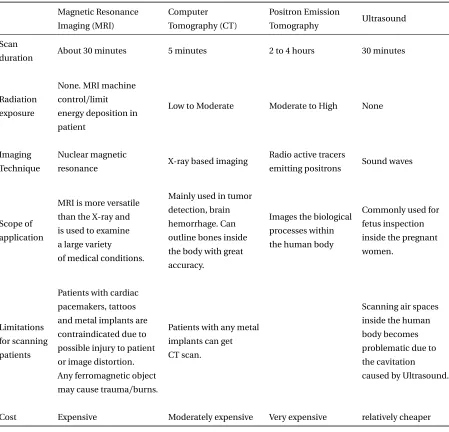
the technique employed. The following table presents a comparative analysis on various types of modalities:
Table 1.1 Table comparing various imaging modalities
Magnetic Resonance Imaging (MRI) Computer Tomography (CT) Positron Emission Tomography Ultrasound Scan
duration About 30 minutes 5 minutes 2 to 4 hours 30 minutes
Radiation exposure
None. MRI machine control/limit energy deposition in patient
Low to Moderate Moderate to High None
Imaging Technique
Nuclear magnetic
resonance X-ray based imaging
Radio active tracers
emitting positrons Sound waves
Scope of application
MRI is more versatile than the X-ray and is used to examine a large variety of medical conditions.
Mainly used in tumor detection, brain hemorrhage. Can outline bones inside the body with great accuracy.
Images the biological processes within the human body
Commonly used for fetus inspection inside the pregnant women.
Limitations for scanning patients
Patients with cardiac pacemakers, tattoos and metal implants are contraindicated due to possible injury to patient or image distortion. Any ferromagnetic object may cause trauma/burns.
Patients with any metal implants can get CT scan.
Scanning air spaces inside the human body becomes problematic due to the cavitation
caused by Ultrasound.
1.1. Artefacts in MR imaging systems
In the scope of this thesis, MR imaging and the corresponding artefacts have been discussed. Like any other imaging modalities, MRI is also limited by artefacts. These artefacts are generally
presented by the MR scanner hardware itself or from the patient interaction with this hardware. As
a result, these artefacts are elevated as abnormalities in the captured images. The following section discusses about the most common types of artefacts observed in MRI systems.
1.1
Artefacts in MR imaging systems
Some of the most commonly observed artefacts in the MR images include truncation artefacts (I),
aliasing artefacts (II), and motion artefacts (III).
1.1.1 Truncation artefacts
Truncation artefacts, also known as ringing artefacts, occur near high-contrast boundaries. These are reflected as a series of lines in the MR image parallel to abrupt intensity changes in the object at this
location. These artefacts are predominantly caused due to the finite sampling of the signal. At high
contrast boundaries in the given image, the Fourier transform (k-space in the context of imaging) corresponds to an infinite number of frequencies, and since sampling is finite, the discrepancy
appears in the image in the form of a series of lines. These artefacts are typically compensated by
changing the sampling frequency in the frequency direction and the number of phase encoding steps in the phase direction. Details about frequency and phase encoding are presented in chapter 2.
Additionally, use of smoothing filters will reduce the sharp transitions in the images by introducing
blur and can be used to reduce these artefacts. Reducing the sharp transitions while maintaining the image quality is an important aspect of the image restoration process involving truncation artefacts.
In lieu with this, Archibald & Gelb[AG02]have proposed using Gegenbauer reconstruction method (a type of smoothing filter) to reduce these ringing artefacts. Other smoothing filters that could be
used are 2-D exponential filters. Further, fat supression techniques are also known to reduce these
ringing artefacts.
1.1.2 Aliasing artefacts
Aliasing artefacts, or wrap around artefacts mainly occur when the Field of View (FOV) is smaller than
the body-part being imaged. The part of the body that lies beyond the edge of the FOV is projected
on to the other side of the image[KBF15]. This phenomenon is usually observed when the data is undersampled. Therefore, these artefacts can be corrected by oversampling the data. Additionally,
1.1. Artefacts in MR imaging systems
continuous MR signal picked by the receiver coil is converted into its digital counterpart and presented as a gray scale image. To obtain high precision conversion, the signal is usually sampled
at a higher rate than the Nyquist frequency. Given the constraints in the MR imaging hardware,
this could lead to longer scan durations, particularly if the k-space is sampled in a cartesian grid. Tsai & Nishimura[TN00]have suggested a variable-density k-space sampling method to reduce
aliasing artefacts in MR images. Their method is based on the assumption that most of the energy
is concentrated around the k-space center (dc frequency values in the fourier space) and that oversampling this region while undersampling the outer k-space region will not contribute severe
aliasing artefacts.
1.1.3 Motion artefacts
The above mentioned type I and II artefacts are usually caused because of the limitations of
hard-ware/software and can be relatively easily compensated. Motion artefacts are mainly caused by
breathing, cardiac movement, blood flow and also the patient’s movement. The involvement of the patient’s physiological processes makes these artefacts relatively difficult to model. The motion of
an entire object during the imaging sequence generally results in the blurring of the captured image
with ghost images in the phase encoding direction. Motion artefacts are easy to distinguish from the truncation artefacts because they extend across the entire Field of View (FOV). Also, unlike the
truncation artefacts, they diminish quickly away from the boundary from which they are originated.
One way to account for these artefacts is by breath-holding techniques, reducing the scan duration in order to capture minimum amount of motion from the patient. Other simpler measure could be
to average the signal in order to get rid of these artefacts. However, these measures result in poor
resolution of the images/discomfort to the image data. Further, in scenarios such as MRI guided PET imaging which usually take longer acquisition time, breath-holding techniques cannot be applied.
A variety of methods have been proposed in the literature to compensate for motion correction.
Some of these methods such as center-out imaging methods e.g., projection-reconstruction[GP92] and spiral MRI[Ahn86]have been shown to reduce these artifacts. These methods are analogous to
the process of over sampling of the central k-space and averaging the same to reduce the artefacts.
Advanced methods for modelling motion related artefacts include measuring the physiological signals (respiratory rate, blood flow rate etc.) related to motion. These physiological signals are
usually measured using external sensors (e.g., respiratory belts, cameras), navigator echoes (mod-ifications within the MR imaging protocols) for tracking motion related signals[Shi00] [Lau13].
Respiratory signal (motion) tracking is also done by using self gating techniques. The respiratory
1.2. Scan duration & the problem of undersampling
of the image captured at various times. Typically, this model is manifested as displacement vector fields describing the nonrigid deformation that maps MRI voxels between different respiratory
states. This type of signal tracking is getting increasingly popular given its simplicity and the fact that
it requires minimal architecture to model the tracking signal. A comprehensive review of the state of the art methods that are used to model the respiratory motion has been presented in[McC13]
and[Gri15]. Motion artefacts are discussed at length in Chapter 2.
1.2
Scan duration & the problem of undersampling
Most of the artefacts that are observed in the MRI imaging modality are a result of undersampling of
the k-space. The problem of undersampling is usually acknowledged when the scan durations are shortened (to facilitate the patient’s comfort). Typical scan durations range for about 5-7 minutes
of duration which account for the TR duration (time taken by the excited nuclei to return back to
the original state) as well as the k-space encoding. Center-out imaging methods which employ radial/spiral k-space sampling are better in the sense that the central k-space portion is very well
sampled when compared to the traditional cartesian sampling methods. To further optimize the scan
duration while acknowledging the problem of undersampling, a golden angular (∆Φ=111.246o) based k-space encoding has been proposed in[Win07]. It has been shown that the golden angular
based increments are related to the Fibonnaci series and can quickly span the entire k-space in
minimal number of encoding steps. This method of k-space encoding has often been referred to as the stack-of-stars framework. Revisiting our motion artifact correction frame work, motion tracking
using self gating techniques accommodating stack of stars framework of gated MR imaging has
been proposed in[Gri15]. However, the effects of aliasing due to the golden angular sampling have not been noted thoroughly in modelling the respiratory tracking signal. This thesis investigates
the effects of aliasing due to the golden angular sampling. We propose a radial k-space encoding
scheme with sub-golden angular increments which are optimal in terms of reducing the aliasing artefacts in the respiratory band width, and also better in terms of scan duration when compared to
the traditional k-space encoding schemes such as cartesian/sequential radial sampling methods.
This thesis is segmented into five chapters. Chapter 1 gives a brief introduction to the MR imaging, the problems posed in the image reconstruction and the proposed solutions to overcome them.
Chapter 2 provides the methods and background needed to investigate this problem. Chapter 3 evaluates the effect of angular sampling with respect to the respiratory tracking signal in a temporal
perspective. Chapter 4 investigates the same from spatial perspective by validating the proposed
CHAPTER 2
BACKGROUND AND METHODS
Chapter 1 has given introduction to MR imaging and listed the advantages/limitations posed by this modality. In particular, it has pointed out on one of the major limitations concerning this
modality, i.e., image deformations due to respiratory motion. Further, it essayed the list of a few
available methods used to overcome the associated limitations. In addition, it has also defined a new limitation, i.e., the problem faced due to the choice of angular sampling in respiratory
track-ing signals. This chapter draws references to the MR imagtrack-ing concepts mentioned in[PL06]and
provides the necessary background needed to understand the functionality of MRI and also gives a comprehensive idea about how the images are acquired using MRI. Section 2.1 explains the physics
behind MRI. In section 2.2, details about the way MR images are acquired have been presented.
Section 2.3 talks about modelling the respiratory signal from the MR images.
2.1
Magnetic Resonance Imaging - Concepts
The concept of Magnetic Resonance Imaging (MRI) arises from the Nuclear Magnetic Resonance property exhibited by some atomic nuclei. Nuclei of the atoms are comprised of protons and
neutrons which make them positively charged. Further, associated with their atomic number ( sum
of the number of protons and neutrons) is the spin of these nuclei, which results in the angular momentumΦ. The spin of these nuclei can be analogically thought of as the movement of charges
2.1. Magnetic Resonance Imaging - Concepts
magnetic moment vector for these individual nuclei is given by:
µ =γΦ (2.1)
whereγis the gyro-magnetic ratio, unique to the atomic nuclei of the atoms. In the whole body
MR imaging, the nuclei of1H - being present in large concentrations within the body because of the water content - are primarily responsible for generating a strong NMR signal. In the resting
state condition, the net magnetic field generated in general is cancelled out due to the random
orientations of the spins of the bulk of these nuclei. In the presence of external magnetic field, depending on the magnitude of the field, these nuclear spins can be made to align to a particular
orientation. The corresponding bulk magnetization vector (M) is given by
M=
Ns
X
i=1
µi (2.2)
For an applied external static magnetic fieldB(t)=Bozˆ, the bulk magnetization vector stabilizes over a period of time and reaches to an equilibrium valueMo:
Mo=
Boγ2h2
4k T PD (2.3)
where h, k, PD are Planck’s constant, Boltzmann’s constant and proton density respectively. In general, the magnetization vectorMis defined in a spatio-temporal dimension, i.e,M=M(r,t). The temporal changes inM(r,t)are governed by the equation:
dM(t)
d t =γM(t)×B(t) (2.4)
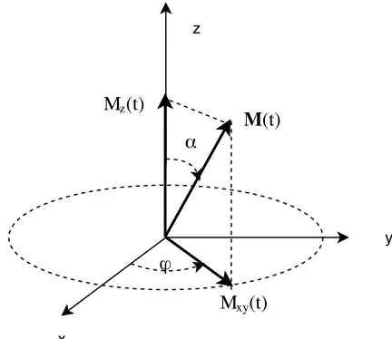
Solving forM(t) from the above equation gives way to the transverse and longitudinal magnetizations Mx y(t) =Mx(t) + jMy(t)and Mz(t)respectively where:
Mx(t) =Mosin(α)cos(−γBot +ϕ)
2.1. Magnetic Resonance Imaging - Concepts
Figure 2.1 Figure illustrating the magnetization vector
whereαis the angle with which the magnetization vector precesses around the z-axis andϕis
an arbitrary angle specifying the initial position of the vector in the transverse plane. The frequency at which the magnetization vector precesses around the magnetic fieldBo in the transverse plane is called Larmor frequency. It is defined as:
2πνo=γBo (2.6)
From the above equation 2.6, theoretically it can be said that the precision frequencyνo is constant
given the right hand side. However, in practical scenarios,Bo is known to fluctuate. Three primary sources addressing this concern are:
• Magnetic field inhomogeneities which arise due to the design of the main magnet
• Magnetic susceptibility - property of the material that increases or decreases the magnetic field within the material relative to the surrounding field.
• chemical shift - the measure of the change in Larmor frequency due to the chemical
2.1. Magnetic Resonance Imaging - Concepts
2.1.1 RF excitation
The transverse magnetized signal Mx y rotates with an angular velocityγBoin the complex xy plane to create a Radio Frequency (RF) excitation in the sample which is recorded for use in the MRI. This
excitation induces time dependent voltage in a coil of wire placed outside the sample and thus manipulates the nuclear spin systems - based on Faraday’s law of induction. However, as soon as the
effect of the induced emf wears off, the magnetization vectorM(t) begins to precess about the z axis which has a much larger field strengthBo. In order to minimize this effect and to get the maximum transverse magnetized signal (Mx y), quadrature RF coils are used to generate circularly polarized RF
excitations which push the bulk magnetization vector back into the transverse plane thus leading to a forced precession of the same. The magnetic field responsible for circularly polarized RF excitations
in the transverse plane (xy) is modelled by:
B1(t) =B1e(t)e−
j(γBot−ψ) (2.7)
whereB1e(t)is the envelope of the RF coil induced magnetic field (2.5) andψis the corresponding initial phase. The final orientation of the magentization vectorM(t) is determined by the amplitude and duration of theB1e(t). Since the RF excitation pulse causes changes in the orientationαof the magnetization vector, it is often referred to as anα-pulse. The final tip angle is related to an RF
excitation pulse of durationτp by :
α=γ
Z τp
0
B1e(t)d t (2.8)
2.1.2 Relaxation
In an ideal scenario, after the RF pulses (α 6= π) are applied, the bulk magnetization vectorM(t) will continue to precess about the main magnetic fieldBoleading to a continuous recording of the signals from the sample. In practice, this is interrupted by relaxation processes (T1 and T2) which together cause the measured signal to vanish. These processes are also known as Longitudinal (T1)
and Transverse (T2) relaxations respectively.
2.1.2.1 Transverse Relaxation
Transverse relaxation (T2), also known as spin-spin relaxation is caused by the perturbations in the magnetic field due to the nearby spins. As a result, the transverse magnetization vector is randomly
2.1. Magnetic Resonance Imaging - Concepts
signal decay also called as Free Induction Decay (FID). The corresponding time constant is denoted byT2. The correspondingMx y(t)then becomes:
Mx y(t) =Mx + j My =Mos i nαe−j(γBot−ϕ)e−t/T2 (2.9)
The following figure illustrates the same:
Figure 2.2 Figure illustrating the de-phasing of the magnetization vector during Transverse relaxation.
In practical scenarios, the perturbations in the static magnetic fieldBo along with the Free Induction Decay, cause the signal to decay faster. These perturbations cause the precision of some
spins to speed up and others to slow down which results in a phenomenon calledspin echoes. This phenomenon is modelled by a first order decay process with time constantT20. As a result, the new time constant for the Transverse relaxation then becomes (T2∗), where:
1 T2∗ =
1 T2+
1
T20 (2.10)
2.1.2.2 Longitudinal Relaxation
Longitudinal (T1) relaxation is a process in which the net magnetization (M) grows/returns to its
initial maximum value (Mo) parallel toBo. The corresponding time constant is denoted byT1. Forα
pulses (α 6= π), the longitudinal magnetization vector is modelled as:
Mz(t) =Mo(1−e−t/T1) +Moc o sαe−t/T1 (2.11)
2.1. Magnetic Resonance Imaging - Concepts
following figure illustrates the effect of longitudinal relaxation on the magnetization vector:
Figure 2.3 Figure illustrating the effect of Longitudinal relaxation.
In general, the longitudinal relaxation effect lasts longer than transverse relaxation effect
-T2 ≤ T1. For most of the whole body imaging the relationship betweenT1andT2usually follows
the inequality 5T2 ≤ T1 ≤ 10T2. In general, the differences in these time constants are reflected
in the intensity of the image captured thereby leading to different contrast mechanisms. The two
dominant types of tissues in the human brain, the gray matter (GM) and the white matter (WM) respond with different excitations by manipulating these time constants.
2.1.3 Bloch Equations
Including the effects of transverse and longitudinal relaxations, the equation 2.4 now becomes:
dM(t)
d t =γM(t)×B(t)−R{M(t)−Mo} (2.12) where
B(t) =Bo +B1(t)
R=
1
T2 0 0
0 T1
2 0
0 0 T1
1
The above set of equations are called Bloch equations. These equations are used to model the behaviour of magnetization vectors during excitation. The behaviour of the NMR signal can be
2.2. Data Acquisition and Spatial position encoding
2.2
Data Acquisition and Spatial position encoding
The previous sections discussed about generating an NMR signal by applying external magnetic
field, and also regarding stabilizing the generated signal for maximizing the measured signal. Given the NMR signal generated from a particular location of the imaging object, this particular section
deals with encoding all such signals generated from an object and thus in generating an MR image.
In the paragraphs to follow, a brief introduction to the architecture of the MRI scanner, spatial encoding of the NMR signals have been discussed.
Architecture of the MRI scanner
A typical MRI scanner consists of five principal components: (1) main magnet - to provide the static Bo magnetic field; (2) a set of (x,y,z) gradient coils to provide a switchable gradient in the main magnetic field - to encode for spatial position in MR data acquisition; (3) resonators or coils for
the transmission and reception of RF pulses - to measure the response from the excited tissues; (4) electronics for programming the timing of transmission and reception of signal; (5) a console
for processing the images. The gradient coils play a crucial role in encoding spatial position by
operating at the Larmor precision frequency (eq:2.6) as well as manipulating the phase of the transverse magnetization vector.
2.2.1 Spatial co-ordinate system
Typically in the MR imaging, the conventions of the spatial co-ordinate system follow those of the right handed system. The+z is always oriented along the direction of the static magnetic field vector Bo. The+y direction is oriented up and therefore the+x direction should face towards the left in the horizontal plane. In terms of the human body anatomy,+z is oriented in the direction from the head to the feet;+y is oriented from the back to the front and+x from the right to the left. The spatial position in an MR image is determined by bothfrequency encodingandphase encoding The first component of the spatial position encoding isfrequency encodingand it deals with varying the Larmor frequency as a function of position. This is done by the gradient coils which provide
spatially varying fields. As a result, equation 2.6 then becomes:
2πνo =γ(Bo +G.r) (2.13)
2.2. Data Acquisition and Spatial position encoding
G=(0, 0,Gz)corresponds to the RF excitations in the z-plane. In general, slice encoding depends on three factors namely:
• Strength (slope) of the z-gradient (concerning the above defined co-ordinate system).
• The gradient fieldGz(concerning the above defined co-ordinate system).
• Center of the range of RF frequencies (Larmor frequencies) generated using equation 2.13
Based on the above three parameters, it is possible to account for both the position and thickness of the slices. It should be noted that the thinner slices have fewer nuclei, which makes the NMR signal
smaller. In practice, obtaining thinner slices is a cumbersome procedure as it requires special pulse
sequences and longer imaging times to amplify the NMR signal.
2.2.2 Spatial position encoding
Frequency encoding
Frequency-encoding of spatial position may be used to define location either within the slice or
between the slices. As mentioned before, the signal of interest in MR imaging is the Transverse Magnetization (TM) vectorMx y(t). After accounting for the Finite Induction Decay (FID), the behaviour of the TM vector can be modelled using the equation:
Mx y(t) =Mx y(0+)e−j(2πνot−ϕ)e−t/T2 (2.14)
whereMx y(0+)=Mz(0−)s i nα. During the frequency encoding, the gradient is turned on during the FID, thereby causing the Larmor frequencies to be spatially dependent. As a result, the frequencyνo
in equation 2.14 is modelled by equation 2.13. Further, it is assumed that the slice thickness in the +zdirection is negligible. SoG.rthen becomesGxx +Gyy. The time constantT2is also assumed
to be spatially variant. The response s(t) during an FID under slice selection is given by:
so(t) =A
Z ∞
−∞
Z ∞
−∞
Mx y(x,y; 0+)e−j(2πνot+γGxx t+γGyy t)e−t/T2(x,y)d x d y
(2.15)
=A e−j2πνot
Z ∞
−∞
Z ∞
−∞
Mx y(x,y; 0+)e−t/T2(x,y)
e−j(γGxx t+γGyy t)d x d y
The received signal at the RF coil is demodulated with carrier signal of Larmor frequency to yeild the
2.2. Data Acquisition and Spatial position encoding
Fourier transform (F(u,v))of the function f(x,y)=Mx y(x,y; 0+)e−t/T2(x,y), also known as effective spin density, with
u = kx=2πγGxt (2.16)
v =ky =2πγGyt
Therefore, the signalso(t)=F(u,v) reads out the information in the trajectory corresponding to the orientation
θ=t a n−1(Gy Gx)
(2.17)
in the polar co-ordinate system. Thus it can be said that MRI reconstructs an image of the effective
spin density f(x,y) of the nuclear systems when placed in external magnetic field. Further,
accom-modating the gradient fields to vary the value ofθscans the k-space of the given object. However, it must be noted that since (t ≥0), the frequency encoding only accounts for the values of (u,v≥0). Remembering that the positive and negative k-space differs only in the phase, the above result
implies the phase loss in the k-space.
Phase encoding
In order to account for the phase loss, the pulse sequence includes the usual slice-selective RF pulse by choosing the band of precision frequencies followed by refocussing the gradient signal to
produce negative gradient field. This way the gradient field becomes
u =kx=−2πγGxt (2.18)
v = ky =−2πγGyt
and captures the values of (u,v ≤0) as well. Once the frequency and the phase information is obtained, the image can be reconstructed using the inverse Fourier transform.
k-space sampling
In the previous section it has been observed that, by choosing spatially variant gradient fields and
also by changing their directions (for phase encoding), it is possible to scan the entire k-space
represented by the object. Further equation 2.17 implies that the signal acquired is along a particular
2.3. Respiratory signal tracking
keeping the productGzz constant and manipulating the other gradient coils. In general, the choice of the sampling scheme depends on the spatial nature of the gradient field (G) generated by the gradient coils. The following figure illustrates the radial sampling of the k-space:
Figure 2.4 Figure illustrating the stack of stars sampling scheme. Hereθ=∆Φt
However, introducing the spatial variability in gradient fields also results in smaller NMR signals
at farther locations thus defining a Field Of View (FOV) for a particular gradient coil. In order to
overcome this limitation, multiple gradient coils (channels) are combined together and used to produce a uniform spatial variant gradient field. The NMR signalssi(t), where i=1,2...N (number of gradient coils), are then combined to reconstruct the image.
2.3
Respiratory signal tracking
One of the major limitations of the MRI is the motion of the patients which results in image
defor-mations. In conventional MR imaging which is the Fourier transform (FT) of the k-space data, the summation operations in the discrete FT imply that each image pixel is composed of a weighted
sum of every point in k-space and vice-versa. Thus, any changes in the pixel intensities caused
by the motion can potentially affect the acquired image. To overcome this, a variety of methods have been proposed in the literature. Although a most rudimentary way to tackle this problem is by
2.3. Respiratory signal tracking
include navigator echoes based corrections, external sensor based corrections and self gating based respiratory signal tracking. In this particular section, a comprehensive study of respiratory tracking
using these three methods is presented. In particular, motion correction using self gating methods is
discussed in detail as it does not need any external architecture, and more importantly it is relevant in the scope of this thesis.
External sensor based motion compensation
External sensors are used to augment the MRI hardware setup. They can provide additional infor-mation with no compromise to the scan sequences or imaging. Optically tracked markers or active
markers albeit not being able to track the internal movements of the tissues are used for motion
compensation[Zai06],[Qin09],[Ooi09]. In these systems, a visible target marker is placed on the object to be imaged. The in-bore video tracking system is then used to evaluate for prospective
motion correction. The movement of the visible target marker is used to generate the motion signal
which is further used in correcting the deformations in the MR images. Alternatively, ultrasound based techniques[Fei10]are also used to monitor the internal motion of the organs in order to
correct the MR images.
Navigator echoes
Navigator echoes[EF89],[Uri07],[Odi10]are usually an additional measurements (FR-pulses) within
the MR imaging sequence, rather than an external measurement such as external sensors. Navigator pulses may be either spin echo or gradient echo. The term navigation refers to inferring some
components of motion from MR data. In its simplest form, navigation is used to acquire extra
non-phase encoded lines of k-space. The Fourier transform of these navigator echoes give projections through the object from which some components of motion can be inferred. In imaging diaphragm,
lungs region, the signal from a cylindrical or ’pencil beam’ shaped excitation through the diaphragm
is measured. The liver/lung border provides good contrast and is relatively easier to track the motion the diaphragm. The echo signal returned by these beams is reconstructed in the direction of motion
and displayed as lines of data along the beam direction.
Self-gating methods
Self-gating methods possess advantages over other methods such as respiratory belts and navigator
echoes as they account for free-breathing, patient’s comfort and do not require any additional
2.3. Respiratory signal tracking
self-gating approach. This approach computes the total intensity of the acquired image at any given time and uses the change in intensity level to model the respiratory signal. In order to accurately
capture the intensities (corresponding to the central k-space), radial sampling methods are usually
preferred. The breathing motion is usually measured from (Kx,Ky,Kz)=0. In the cases where the central k-space (cksp) is used, the projections (on the axis passing from foot to head) of the Fourier
transform of the cksp volume are used[Bue12]. Further, each of the intensity values/projections
obtained from the origin/cksp are compared with a reference value/projection (total intensity/ projection captured at the end of the respiratory cycle) to generate the respiratory tracking signal.
In lieu with this line of thought, correlation coefficient maximization has been proposed in[Bue12].
This metric is defined as:
C C =
PNr d
i=1(ri−r¯)(pi−p¯)
Ç PNr d
i=1(ri−r¯)2
PNr d
i=1(pi−p¯)2
(2.19)
whereri andpiare the individual pixel intensities of the given projection, ¯r and ¯pare the average intensity values for the corresponding projections,Nr d is the total number of reconstructed pixels in the readout direction. The obtained signal is then passed through a band-pass filter (0.3 - 0.7 Hz)
to get rid of any unwanted artifacts other than the respiratory signal. The signal is then binned into
bins of various sizes weighted by the most commonly occuring phase in the respiratory signal. In particular, it is observed that this phase occurs near the peak of the signal[Bue12].BH Q is the bin corresponding to this phase and can be seen in the figure 2.4. The radial k-space readouts (spokes)
are then sorted into the respective bins in order to reconstruct the images that correspond to these respiratory positions. All such generated images are co-registered in order to compute the motion
fields that could account for the deformations caused due to motion artefacts such as respiration.
2.3. Respiratory signal tracking
Figure 2.5 Figure illustrating the respiratory signal tracking procedure. Source : Buerger et al.[Bue12]
Summary
To summarize this chapter, we have learnt that:
• MR imaging is based on the phenomenon of nuclear magnetic resonance which is a property
exhibited by the atomic spin systems.
• The spin systems are manipulated in presence of external magnetic field and get magnetized in bulk over the time.
• The equations of the motion for this magnetized vector are governed by the Bloch equations which account for Transverse relaxation and longitudinal relaxation parameters
• These equations describe a precession of the magnetization vector around the external
mag-netic field directionBozˆwith Larmor frequency.
• An RF pulse will cause the magnetization vector to precess around the external magnetic field.
• The observed signal in MRI is an RF pulse produced by the rapidly rotating transverse
magne-tization
• By influencing the proton density with T1 and T2 weighting mechanisms, different contrast
images are generated.
2.3. Respiratory signal tracking
• By manipulating the gradient fields (Gx,Gy,Gz) one can access the entire k-space of the object in various frameworks (e.g: stack of stars (cylindrical), cartersian, spherical, spiral etc.)
• Motion artefacts in MR imaging cause deformations in the generated images and are
CHAPTER 3
EVALUATION OF ANGULAR SAMPLING
WITH RESPECT TO THE RESPIRATORY
TRACKING SIGNAL
In chapter 2, we have discussed about the background and the concepts related to the MR imaging.
We have learnt about some of the limitations of this imaging modality and also about the proposed
methodologies to overcome the same. In particular, we have studied the respiratory signal modelling using external sensor based, navigator echoes based and self-gating methods. Following the results
obtained for golden angular sampling in being able to quickly scan the entire k-space Winkelmann
et al.[Win07], this choice of angular sampling has been preferred for self-gated respiratory signal tracking frameworks in studies conducted by Grimm et al.[Gri15], Buerger et al.[Bue12]. In this
chapter, we evaluate the effects of the choice of the angular sampling with respect to the
respira-tory tracking signal. The sections to follow will present the analysis on various choices of angular increments (sequential, sub-golden, golden & random) and their effects on the respiratory tracking
signal.
Data Acquisition
In dynamic radial MR image reconstruction using the Stack of stars approach, the k-space is divided
figure 2.4. The k-space is filled by these profiles over a period of time. All such acquired profiles are reconstructed to form an MRI image, which is discussed extensively in the chapters to follow (4.1).
The choice of the azimuthal angular sampling puts a constraint on the total area spanned in the
k-space and thereby constraints the data acquisition time. Winkelmann et al.[Win07]have shown that an angular spacing of(∆Φ)=111.246 is efficient in image reconstruction as it spans the entire
k-space with minimal number of read outs along each azimuthal profile. In tracking the respiratory
signal using self gating framework, the total intensity captured at the dc frequency is used as an indirect metric to determine the changes in the soft tissue during respiratory cycles (inhalation and
exhalation). In order to focus on the respiratory artefacts, MRI data from water filled phantom was
chosen as it does not exhibit any signs of respiration. Thus, any changes in the frequency spectra can be clearly attributed to the artefacts that are the result of the profile spacing (∆Φ) and the
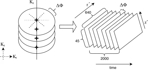
data acquisition procedure of the imaging system. The dataset has been recorded usingSiemens Biograph mMR scannerwith5active channels. The 4-D k-space (r ∈ {−R2,
R
2},θ,z,t) here, is a
warped 3-D whereθ andt are collapsed into a single dimensionθ(t) = ∆Φ× t. The k-space of the phantom data has been sampled at (640 X 45) complex data points along each azimuthal profile
(a spoke in 2-D plane), and it consists of 2000 such profiles acquired at 5 profiles every second. The spacing between each profile (∆Φ) for this data collection was set to be 111.246o, based on the
golden angle[Win07]. The origin of the k-space as provided by the metadata of the MR image is located at the slice r=320 and z=17 (r=321 and z=18 for matlab).
Figure 3.1 Figure illustrating the data acquisition
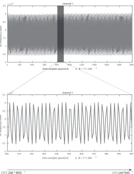
The following figure shows the 2000 spokes acquired from the slice 18 (z=0 plane) and slice 321
0 200 400 600 800 1000 1200 1400 1600 1800 2000
time samples spaced at ∆Φ = 111.246 o 6 6.5 7 7.5 8 8.5 9 9.5
dc frequency value
×105 channel 1
800 810 820 830 840 850 860 870 880 890 900
time samples spaced at ∆ Φ = 111.246 o
6 6.5 7 7.5 8 8.5 9 9.5 dc freq ue n cy v alue
×105 channel 1
o o time samp time samp time time 5 10 × 1000 1000 ∆ ΦΦ
(111.246 * 800) (111.246*900)
Figure 3.2 A sample figure illustrating the intensities of the dc frequency component (slice : 321, r=0; slice
: 18, z=0 ) of channel 1 captured for 2000 readouts at different angles (spokes) (each spoke ’n’ is oriented
at an angle∆Φn)
The 2000 spokes correspond to an angle (θ= (∆Φt)≥ 0) were sorted into the true angles. A true angle is defined as follows:
θtrue=θ(t)% 360 (3.1)
= (∆Φt) % 3601 (3.2)
where % is the modulo operator. Further, the intensities at the dc frequency component has been
1The modulo should ideally be operated at 180 given (r ∈ {−R
2,
R
2}). However, in general, the readout direction from
({−R2 −→
R
2}) is not the same as from ({
R
2−→ −
R
2}). This is attributed to various factors like phase encoding, gradient coil
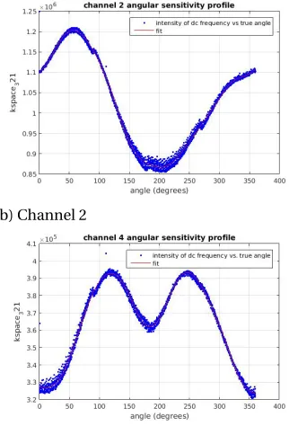
calculated as a function of the true angle. The following figures show the dc frequency intensity vs true angle characteristics for each of the five channels.
(a) Channel 1 (b) Channel 2
(c) Channel 3 (d) Channel 4
(e) Channel 5
Figure 3.3 Angular sensitivity profiles of the given channels.
In an ideal case, the dc frequency should not change with the true angle implying that the
angular sensitivity profile is a straight line (and a perfect circle in the k-space near origin). However,
The above distributions of each channel’s dc frequency profile with respect to the true angle were mathematically modelled by fitting curves using fourier series. Once the models were constructed
for each channel, they were used to resample the phantom data for each channel at different desired
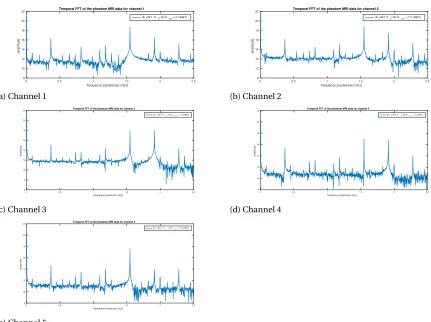
angular increments. Having generated the data sequence, the temporal fourier transform of the sequence is further used to compute the signal power in the respiratory band (0.3 - 0.7 Hz). Given
the phantom dataset, any undesirable peaks in the respiratory band width can be attributed to the respiratory artefacts. The slice (Kr=321Kz =18) was used in order to compare the effect of artefacts caused by each angular increment in the respiratory band of the signal. The following
figures show the temporal frequency spectrum of a dynamic MR imaging system acquired at the
angular increments of(∆Φ)=111.246 degrees.
0 0.5 1 1.5 2 2.5
frequency [cycles/sec (Hz)] 8 10 12 14 16 18 20 22 amplitude
Temporal FFT of the phantom MRI data for channel 1
(Kr=321, Kz=18, Kθ (t)=111.246*t)
(a) Channel 1
0 0.5 1 1.5 2 2.5
frequency [cycles/sec (Hz)] 8 10 12 14 16 18 20 22 amplitude
Temporal FFT of the phantom MRI data for channel 2
(Kr=321, Kz=18; Kθ (t) = 111.246*t)
(b) Channel 2
0 0.5 1 1.5 2 2.5
frequency [cycles/sec (Hz)] 6 8 10 12 14 16 18 20 22 amplitude
Temporal FFT of the phantom MRI data for channel 3
(Kr = 321, Kz = 18, Kθ (t) = 111.246*t)
(c) Channel 3
0 0.5 1 1.5 2 2.5
frequency [cycles/sec (Hz)] 8 10 12 14 16 18 20 22 amplitude
Temporal FFT of the phantom MRI data for channel 4
(Kr) = 321, Kz = 18, Kθ (t) = 111.246*t
(d) Channel 4
0 0.5 1 1.5 2 2.5
frequency [cycles/sec (Hz)] 8 10 12 14 16 18 20 22 amplitude
Temporal FFT of the phantom MRI data for channel 5
(Kr = 321, Kz = 18, Kθ (t) = 111.246*t)
(e) Channel 5
3.1. Effect of artefacts due to angular sampling with sequential increments of1o
The above figures show the temporal FFT spectrum of spatial dc component of the the phantom dataset. In what should have been an ideal scenario, the FFT spectrum should have been aδfunction
with peak at dc temporal frequency2. However, the above figures showcase the presence of artefacts
in the signal. From the above figures, it can be seen that there is a predominant peak in the respiratory bandwidth (0.3 - 0.7 Hz). These artefacts are primarily due to the sensitivity of the channels due to
the limitations on their field of view, and also due to the effects of the angular sampling. Accounting
for the channel sensitivity artefacts is a tough task to pursue, as it requires modelling the channel sensitivity maps (in 3-D k-space). Further, the channel sensitivity maps are difficult to measure with
a patient in the scanner. However, the effects of angular sampling can be accounted for, by creating
the angular sensitivity models of the individual channels and further use them to sample the data at desired angular increments. In this line of thought, the angular sensitivity fits generated for all the
five channels were sampled at various angular increments in order to study the effect of the angular
sampling artefacts. Three types of sampling were used to study these artefacts.
3.1
Effect of artefacts due to angular sampling with sequential
incre-ments of
1
oIn this section, the angular sensitivity models generated for each of the respective channels were
sampled at consecutive 1o angular increments. Further, the temporal FFT of the sampled data from
the models for all the MRI channels was compared with the temporal FFT of the original data. The following figures show the FFT comparisons of the same:
3.1. Effect of artefacts due to angular sampling with sequential increments of1o
0 0.5 1 1.5 2 2.5 frequency [cycles/sec (Hz)]
8 10 12 14 16 18 20 22 amplitude
Actual vs modelled respiratory tracking FFT profiles - Channel 1
original reconstructed at the increments of 1 o
(a) Channel 1
0 0.5 1 1.5 2 2.5 frequency [cycles/sec (Hz)]
8 10 12 14 16 18 20 22 amplitude
Actual vs. modelled FFT of respiratory tracking signal for Channel 2
original reconstructed at the increments of 1 o
(b) Channel 2
0 0.5 1 1.5 2 2.5 frequency [cycles/sec (Hz)]
6 8 10 12 14 16 18 20 22 amplitude
Actual vs. modelled FFT of respiratory tracking signal - Channel 3
original reconstructed at the increments of 1 o
(c) Channel 3
0 0.5 1 1.5 2 2.5 frequency [cycles/sec (Hz)]
8 10 12 14 16 18 20 22 amplitude
Actual vs. modelled FFT of respiratory tracking signal - Channel 4
original reconstructed at the increments of 1 o
(d) Channel 4
0 0.5 1 1.5 2 2.5 frequency [cycles/sec (Hz)]
8 10 12 14 16 18 20 22 amplitude
Actual vs modelled FFT of respiratory tracking signal - Channel 5
original reconstructed at the increments of 1 o
(e) Channel 5
Figure 3.5 Temporal frequency spectral comparison of the given channels for reconstruction using 1o
3.2. Effect of artefacts in the respiratory tracking signal due to sub-golden angular increments
From the above figures, it can be observed that sequential sampling does a better job in terms of generating a smooth temporal FFT spectra for each of the respective channels. However, the overall
noise contributed by this sequential sampling method in the respiratory bandwidth (0.3 - 0.7 Hz) is
greater than that of the actual dataset (which was acquired at the increments of the golden angle). Further, it is also necessary to emphasize on the number of samples required by this particular
sampling method in order to scan the entire k-space. It takes about a minimum of 360 time samples
(each as a function of true angle) for this method to cover the entire k-space. Following this result, the effects of the artefacts due to different sampling increments have been analyzed and presented
in the section below.
3.2
Effect of artefacts in the respiratory tracking signal due to sub-golden
angular increments
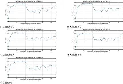
In this section, the angular sensitivity models generated for each of the respective channels were sampled at sub golden angular increments. This choice of angular sampling was preferred in order
to preserve any advantages that golden angular sampling has when compared to other angular
increments. The angular sensitivity models were sampled at angular increments that factorize the golden angle. The angular increments ranged from[0 : 5.5623 : 111.264]( where 5.5623=201 (111.246)).
Further, the power contributed by each of these angular increments in the respiratory bandwidth
3.2. Effect of artefacts in the respiratory tracking signal due to sub-golden angular increments
0 20 40 60 80 100
corresponding angular spacing value [degrees] -5 0 5 10 15 20 25 power [dB]
Respiratory band power for Phantom MRI data - Channel 1
(a) Channel 1
0 20 40 60 80 100
corresponding angular spacing value [degrees] -5 0 5 10 15 20 25 power [dB]
Respiratory band power for Phantom MRI data - Channel 2
(b) Channel 2
0 20 40 60 80 100
corresponding angular sampling value [degrees]
-5 0 5 10 15 20 25 power [dB]
Respiratory band power for Phantom MRI data - Channel 3
(c) Channel 3
0 20 40 60 80 100
corresponding angular sampling value [degrees]
-5 0 5 10 15 20 25 power [dB]
Respiratory band power for Phantom MRI data - Channel 4
(d) Channel 4
0 20 40 60 80 100
corresponding angular sampling value [degrees]
-5 0 5 10 15 20 25 power [dB]
Respiratory band power for Phantom MRI data - Channel 5
(e) Channel 5
Figure 3.6 Respiratory power profile for various sub-golden angular increments for the given channels
From the above figures, it can be observed that the artefacts generated due to angular sampling
at 61.18o and 72.3099o correspond to the lowest power in the respiratory bandwidth (0.3 - 0.7
Hz). It should also be noted that the minimum respiratory artefact power occurs at these angles
3.2. Effect of artefacts in the respiratory tracking signal due to sub-golden angular increments
0 0.5 1 1.5 2 2.5
frequency [cycles/sec (Hz)] 8 10 12 14 16 18 20 22 amplitude
Temporal FFT comparison - Channel 1
original
reconstructed at the increments of 61.18 o reconstructed at the increments of 72.3099 o
(a) Channel 1
0 0.5 1 1.5 2 2.5
frequency [cycles/sec (Hz)] 8 10 12 14 16 18 20 22 amplitude
Temporal FFT comparison - Channel 2 original
reconstructed at the increments of 61.18 o reconstructed at the increments of 72.3099 o
(b) Channel 2
0 0.5 1 1.5 2 2.5
frequency [cycles/sec (Hz)] 6 8 10 12 14 16 18 20 22 amplitude
Temporal FFT comparison - Channel 3
original
reconstructed at the increments of 61.18 o reconstructed at the increments of 72.3099 o
(c) Channel 3
0 0.5 1 1.5 2 2.5
frequency [cycles/sec (Hz)] 6 8 10 12 14 16 18 20 22 amplitude
Temporal FFT comparison - Channel 4 original
reconstructed at the increments of 61.18 o reconstructed at the increments of 72.3099 o
(d) Channel 4
0 0.5 1 1.5 2 2.5
frequency [cycles/sec (Hz)] 6 8 10 12 14 16 18 20 22 amplitude
Temporal FFT comparison - Channel 5
original
reconstructed at the increments of 61.18 o reconstructed at the increments of 72.3099 o
(e) Channel 5
Figure 3.7 Temporal frequency spectral comparison of the given channels for reconstruction using 61.18o
(plotted in red) and 72.31o(plotted in orange) sequential angular increments vs. the original data (sampled
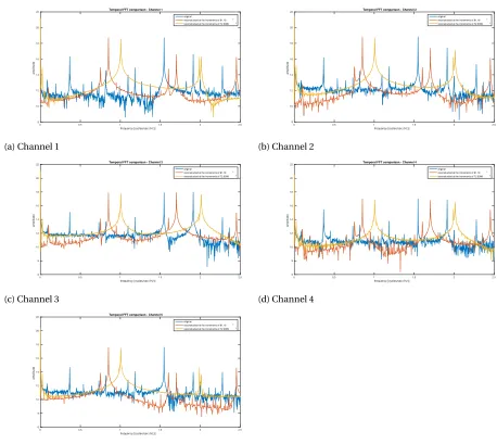
3.2. Effect of artefacts in the respiratory tracking signal due to sub-golden angular increments
It can be observed from the above figures that sampling at these angular increments has not only produced a relatively smoother frequency spectrum for each of the individual channels, but
also minimized the artefacts in the respiratory band. However, the range of k-space spanned by
these angular increments should be considered into account. The following figures display the range spanned by the sub golden angular increments for a given set to time sequence of the radial
samples:
-0.5 0 0.5
-0.5 0 0.5
5.5623
-0.5 0 0.5
-0.5 0 0.5
11.1246
-0.5 0 0.5
-0.5 0 0.5
16.6869
-0.5 0 0.5
-0.5 0 0.5
22.2492
-0.5 0 0.5
-0.5 0 0.5
27.8115
-0.5 0 0.5
-0.5 0
0.5 33.3738
-0.5 0 0.5
-0.5 0
0.5 38.9361
-0.5 0 0.5
-0.5 0
0.5 44.4984
-0.5 0 0.5
-0.5 0
0.5 50.0608
-0.5 0 0.5
-0.5 0
0.5 55.6231
-0.5 0 0.5
-0.5 0
0.5 61.1854
-0.5 0 0.5
-0.5 0
0.5 66.7477
-0.5 0 0.5
-0.5 0
0.5 72.31
-0.5 0 0.5
-0.5 0
0.5 77.8723
-0.5 0 0.5
-0.5 0
0.5 83.4346
-0.5 0 0.5
-0.5 0
0.5 88.9969
-0.5 0 0.5
-0.5 0
0.5 94.5592
-0.5 0 0.5
-0.5 0
0.5 100.1215
-0.5 0 0.5
-0.5 0
0.5 105.6838
-0.5 0 0.5
-0.5 0
0.5 111.2461
Figure 3.8 Range of k-space spanned by different angular increments in 20 readouts of the k-space
Figures 3.8 and 3.9 illustrate the performance of the angular sampling rate in scanning the
k-space of the image. It can be observed that the performance of each of the sub-golden angular
3.2. Effect of artefacts in the respiratory tracking signal due to sub-golden angular increments
-0.5 0 0.5
-0.5 0
0.5 5.5623
-0.5 0 0.5
-0.5 0
0.5 11.1246
-0.5 0 0.5
-0.5 0
0.5 16.6869
-0.5 0 0.5
-0.5 0
0.5 22.2492
-0.5 0 0.5
-0.5 0
0.5 27.8115
-0.5 0 0.5
-0.5 0 0.5
33.3738
-0.5 0 0.5
-0.5 0 0.5
38.9361
-0.5 0 0.5
-0.5 0 0.5
44.4984
-0.5 0 0.5
-0.5 0 0.5
50.0608
-0.5 0 0.5
-0.5 0 0.5
55.6231
-0.5 0 0.5
-0.5 0 0.5
61.1854
-0.5 0 0.5
-0.5 0 0.5
66.7477
-0.5 0 0.5
-0.5 0 0.5
72.31
-0.5 0 0.5
-0.5 0 0.5
77.8723
-0.5 0 0.5
-0.5 0 0.5
83.4346
-0.5 0 0.5
-0.5 0
0.5 88.9969
-0.5 0 0.5
-0.5 0
0.5 94.5592
-0.5 0 0.5
-0.5 0
0.5 100.1215
-0.5 0 0.5
-0.5 0
0.5 105.6838
-0.5 0 0.5
-0.5 0
0.5 111.2461
Figure 3.9 Range of k-space spanned by different angular increments in 50 readouts of the k-space
in both 20 and 50 readouts of the k-space, it certainly is not the best choice of sampling from
the perspective of the respiratory artefacts (figs 3.6a - 3.6e). Having said this, the optimal choices
of angular sampling (61.18o and 72.31o) in terms of the respiratory artefacts are limited by the minimum number of readouts required to span the k-space. This projects the choice of angular
sampling into a 2 dimensional frame work (the 2 dimensions being : Minimum number of readouts
3.3. Effects of artefacts in the respiratory tracking signal due to random angular increments
3.3
Effects of artefacts in the respiratory tracking signal due to random
angular increments
In the following section, the effects of artefacts in the respiratory signal have been analyzed when the k-space of the image is sampled at random angular increments. For this particular analysis,
2000 readouts, each of them corresponding to a random angular orientation have been generated
from the modelled angular sensitivity fits of each of the channels. The random angle sequence has been generated in between (0 - 360) using
randi
, Matlab. The distribution profiles of such randomangular increments for different number of readouts in the k-space has been plotted below:
-0.5 0 0.5
-0.5 0
0.5 10
-0.5 0 0.5
-0.5 0
0.5 20
-0.5 0 0.5
-0.5 0
0.5 50
-0.5 0 0.5
-0.5 0 0.5
70
-0.5 0 0.5
-0.5 0 0.5
90
-0.5 0 0.5
-0.5 0 0.5
120
-0.5 0 0.5
-0.5 0
0.5 150
-0.5 0 0.5
-0.5 0
0.5 170
-0.5 0 0.5
-0.5 0
0.5 200
3.3. Effects of artefacts in the respiratory tracking signal due to random angular increments
The following figures show the temporal frequency spectrum of the k-space reconstructed with random angular increments for 2000 readouts of the k-space and compare it with the original data:
0 0.5 1 1.5 2 2.5
frequency [cycles/sec (Hz)] 8 10 12 14 16 18 20 22 amplitude [dB]
Temporal FFT comparison - Channel 1
original
reconstructed at random angular increments
(a) Channel 1
0 0.5 1 1.5 2 2.5
frequency [cycles/sec (Hz)] 8 10 12 14 16 18 20 22 amplitude [dB]
Temporal FFT comparison - Channel 2
original
reconstructed at random angular increments
(b) Channel 2
0 0.5 1 1.5 2 2.5
frequency [cycles/sec (Hz)] 6 8 10 12 14 16 18 20 22 amplitude [dB]
Temporal FFT comparison - Channel 3
original
reconstructed at random angular increments
(c) Channel 3
0 0.5 1 1.5 2 2.5
frequency [cycles/sec (Hz)] 8 10 12 14 16 18 20 22 amplitude [dB]
Temporal FFT comparison - Channel 4
original
reconstructed at random angular increments
(d) Channel 4
0 0.5 1 1.5 2 2.5
frequency [cycles/sec (Hz)] 8 10 12 14 16 18 20 22 amplitude [dB]
Temporal FFT comparison - Channel 5
original
reconstructed at random angular increments
(e) Channel 5
Figure 3.11 Temporal frequency spectral comparison of the given channels for reconstruction using
ran-dom angular increments (plotted in red) vs. the original data (sampled at 111.246o).
Figures 3.11a - 3.11e show the temporal spectral properties of the k-space scanned using random angular increments. It can be observed that for the same phantom MRI dataset, the overall average
power spectrum generated due to the random angular increments is much higher than the original
power spectrum. Also, the temporal frequency spectra generated by random angular increments appears to be noisier than that of the original dataset. Given the various choices of the angular
3.3. Effects of artefacts in the respiratory tracking signal due to random angular increments
this analysis makes sense iff the quality of the image reconstructed using these angular sampling choices is better/not-worsened when compared to the original image. Having said that, the following
chapter focusses on the spatial frequency characteristics of the k-space of the phantom MRI dataset.
Summary
To summarize this chapter, we have learnt that:
• Golden angular sampling scheme (∆Φ=111.246o) is not exactly optimal in modelling the
respiratory tracking signals - as it gives way to aliasing artefacts in the respiratory signal region
(0.3 - 0.7 Hz)
• Following this result, various angular sampling schemes (sub-golden, random and sequential) have been investigated.
• It has been observed that angular sampling increments of 61.18oabd 72.3099o yield minimal