Sources of variation in leaf shape among two populations of Achillea lanulosa.

(1)

Sources of Variation in Leaf Shape Among

Two

Populations

of

Achillea lanulosa

Jessica Gurevitch

Department of Ecology and Evolution, State University of New York at Stony Brook, Stony Brook, New York 11 794-5245 Manuscript received June 10, 199 1

Accepted for publication October 25, 1991

ABSTRACT

Achillea lanulosa has complex, highly dissected leaves that vary in shape and size along an altitudinal gradient. Plants from a high and an intermediate altitude population were clonally replicated and grown in a controlled environment at warm and cool conditions under bright light. There were genetic differences among populations and among individuals within populations in leaf size and shape. Heritabilities for leaf size and shape characters were moderate. Leaves of the lower altitude population were larger and differed from the higher altitude plants in both coarse and fine shape. Plastic response to temperature of the growth environment paralleled the genetic differentiation between low and high altitude populations. There was no apparent trade-off between genetic control over morphology and the capacity for directional plastic response to the environment. Differences in leaf dissection and size at contrasting altitudes in this species are the result of both genetic divergence among populations and of acclimative responses to local environments.

E

COLOGICAL, morphological and physiological differences among plant populations and species growing along altitudinal gradients have been of en- during interest to students of ecology and evolution (e.g., TURESSON 1922, 1925; CLAUSEN, KECK and HIESEY 1940, 1948; MOONEY and BILLINGS 1961;

SLATYER and FERRAR 1977; KORNER and DIEMER

1987). Diminution in leaf size with increased altitude has been noted for a broad group of herbaceous species (BILLINGS and MOONEY 1968). However, while the adaptive implications of leaf shape differences have been well documented (e.g., RASCHKE 1960;

VOGEL 1970; PARKHURST and LOUCKS 1972; TAYLOR

1975; BALDING and CUNNINGHAM 1976; CAMPBELL

1977; ORIANS and SOLBRIG 1977; GIVNISH 1979; GATES 1980), little is known about genetic variation in shape within and among populations at different altitudes, or about the magnitude of plastic vs. genetic variation in leaf shape.

T h e purpose of the present study was to quantify the sources of variation in leaf morphology within and among two populations of Achillea lanulosa Nutt. (As- teraceae) from contrasting altitudes at warm and cool temperatures. Like many species in the genus, A.

lanulosa has complex, highly dissected leaves. In nature, leaves are larger and more highly dissected at lower altitudes, and smaller, more pubescent, and more compact in shape as altitude increases (GUREV-

ITCH 1988). Previous work demonstrated that there was a genetic basis to the differences among populations in the degree of leaf dissection. Genetic differences within populations also were found to exist, as well as plastic (or acclimative) differences with respect

Genetics 1 3 0 385-394 (February, 1992)

to the light environment (GUREVITCH 1988). One of the most striking differences in the environment as altitude increases in alpine regions are ambient temperatures, although, of course, many other factors also change in concert with altitude. It is well known that leaf shape may change dramatically within a given plant genotype if a leaf is produced in full sun as opposed to shade. Few studies have questioned the effects of growth temperature on leaf shape in non- cultivated plant species, however (but see SMITH and NOBEL 1978). I examined the effects of growing Achillea plants collected from an intermediate and a high altitude site under contrasting temperature re- gimes in a temperature controlled glasshouse in bright light. It has been hypothesized that the differences in leaf shape among populations of Achillea from different altitudes are adaptive, with the more compact leaves of high altitude plants having greater capacity to warm above ambient temperature, while the highly dissected leaves of lower altitude plants should remain close to air temperature (GUREVITCH 1988; GUREV- ITCH and SCHUEPP 1990).

MATERIALS AND METHODS

A. lanulosa is most commonly found in the mountains of the western United States at higher altitudes. In the Sierra Nevada range of California it occurs from ca. 800 to 3350

m altitude (CLAUSEN, KECK and HIESEY 1948). It is a small,

tetraploid ( n = 18) herbaceous perennial native to North America, and has been regarded as part of the Achillea millefolium species complex (CLAUSEN, KECK and HIESEY 1948).

(2)

386 J. Gurevitch

The lower altitude population, Mather, is on the western edge of Yosemite National Park at 1400 m, and the higher altitude population, Timberline, is east of the park at 3050 m. The climate and vegetation at these sites are described elsewhere in detail (CLAUSEN, KECK and HIESEY 1948; GUR- EVITCH 1988). Plants were taken at >2 m apart to maximize the possibility of obtaining genetically distinct individuals. Achillea plants in cultivation reproduce vegetatively from naturally produced rhizomes, and a stock collection of plants was maintained in a glasshouse at Stony Brook over many vegetative “generations” before the experiment was begun. This would minimize any possible carryover of residual environmental effects from the field.

In January 1989 approximately 12 clonal replicates of each of 25 genets (genetic individuals) for each of the two populations were sent bareroot and wrapped in moist paper toweling to the OEB glasshouse at Harvard University. Plants were potted in 1-liter containers and maintained in a common environment for ca. 5 weeks. All leaves were then clipped back (so that new leaves could be identified) and replicates were randomly assigned to a cool or warm glasshouse bay on 3-4 March 1991. Only leaves produced after this time (in practice, well after plants were exposed to experimental treatments) were measured in the experiment. Temperatures were set at 14” day/8” night in the cool bay, and 28” day/20” in the warm bay. As the experiment progressed and outdoor temperatures increased, it became difficult to maintain these temperatures in the glasshouse. By the time the experiment was concluded, midday temperatures were somewhat warmer than the above settings, particularly in the “cool” bay. Supplemental lighting was provided by metal halide lamps for 12 hr per day.

Each bay was divided into six blocks. Replicates of each genet (as available) for the Mather and Timberline populations were assigned at random to each block. Positions within blocks were also randomized. After plants had grown for

ca. 10 weeks in the controlled enviyonments, the most recent fully expanded leaf was harvested.

Experimental design and analysis: The experiment was a mixed model nested factorial design. As the design was unbalanced, approximate F tests were constructed with the

SAS 6 statistical package, using the RANDOM/TEST state- ment in PROC GLM, and employing the Satterthwaite approximation to test hypotheses (MILLIKEN and JOHNSON

1984). This results in fractional approximations for the degrees of freedom in F tests. Unfortunately it was not possible to replicate temperature treatments because only two bays were available for the experiment. One therefore can test only for differences among bays, making the fairly reasonable assumption that the major differences between bays was the temperature setting. The bay (or temperature) effect was essentially tested against variation among blocks within bays. The power for testing differences in temperature effects is consequently low. Other effects, particularly differences among populations and interactions between population and environment, were of greater interest in this experiment and were tested with greater power.

Within each population I determined the proportion of variance accounted for by the main effects and interaction terms. Quantitative genetics experiments ordinarily attempt to account for variance due to genetic and environmental factors, and to the interaction between them (FALCONER

1981). The experimental design in this study allowed a more complete accounting for variance terms than is usual, with large-scale differences due to the environments in the two bays separable from small-scale environmental differences due to position within bays. The proportion of variance accounted for by differences among genets is equiva-

lent to broad sense heritability, which provides an upper limit estimate of additive genetic variance (FALCONER 198 1).

Bay X genet interaction variance describes “norm of reaction” differences among genets in response to the environmental differences in the two bays. Variance among blocks (within bays) is caused by small-scale variation in the environment within bays. Differences among genets in response to this small-scale environmental variation is similar to ordinary genotype-environment interaction variance. Vari- ance that cannot be accounted for is placed in the “error” term. I also calculated the “variance” accounted for by bays, as suggested by FALCONER (1 98 l), although, strictly speak- ing, this was a fixed effect.

Variance components were calculated using two SAS procedures, MIVQUEO (minimum variance quadratic unbiased estimator method; HARTLEY, RAO and LAMOTTE

1978) and REML (restricted maximum likelihood). When an experimental design is unbalanced, as this one was, these methods may give different results. If the results are sub- stantively in agreement, we may assume that they are fairly robust. Unbalanced models can sometimes yield negative estimates of variances. MILLIKEN and JOHNSON (1 984) pro- pose a method for building models which can eliminate these negative estimates. They suggest beginning by fitting the complete model, and if not all variance components are statistically significant, eliminating the least important (that one with the largest estimated significance level in the AN- OVA). The reduced model is then fit. If negative variance components remain, the process is iterated. The variance components that are eliminated are estimated to be equal to zero. I followed a modification of this procedure, in that variance components that were not statistically significant were not eliminated if no negative variance estimates re- mained.

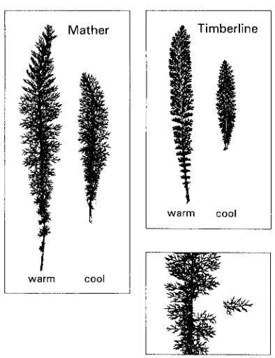
Morphometric measurements and analysis: Morpho- metric data were collected on dried, pressed leaves. Achillea leaves are complex in shape, with primary, secondary, and tertiary leaf segments (or leaflets, Figure 1). It was of interest to characterize both general, or coarse, leaf shape, as well as fine leaf shape. General, basic leaf shape describes the overall dimensions of the leaf outline; for example, the contrast between short, wide‘leaves and long narrow ones. Fine leaf shape, in the case of Achillea leaves, refers to leaf dissection and complexity of shape. Measurements and counts taken included: leaf dry mass, leaf length (including petiole), length of the longest primary leaf segment ( X half leaf width), number of primary segments, length of the longest secondary segment on the longest primary segment, number of secondary segments on the longest primary segment, and number of tertiary segments on the longest secondary segment of the longest primary segment. Meas- urements were log transformed prior to analyses. Trans- formed values for leaf dry mass, leaf length, longest primary segment length, and number of primary segments con- formed reasonably well with ordinary statistical assumptions.

N o satisfactory transformation was found for secondary segment length, number of secondary segments, and number of tertiary segments.

Regression analysis and analysis of covariance (AN-

(3)

warm cool

ri

warm cool

FIGURE 1.-(Left diagram) Digitized image of the first fully expanded leaf from a single genet of a Timberline plant grown in the warm bay (left) and in the cool bay (right). T h e images were produced passing leaves through an optical scanner. T h e larger leaf is approximately 11.5 cm long. (Right diagram) T h e first fully expanded leaf from a Mather genet grown in the warm bay (left) and in the cool bay (right). T h e longer leaf is approximately 20 cm long. (Bottom diagram) T h e central portion of a Mather leaf in the warm bay, enlarged to show details of leaf shape. O n e primary segment has been separated from the main axis of the leaf, and a second primary segment removed from view for clarity. T h e portion shown is approximately 6 cm long.

A second question regarding leaf shape was whether Achillea leaves are composed of self-similar units. That is, is the structure of a primary leaf segment merely a smaller version of the leaf itself, and a secondary leaf segment a miniature of the primary segment? If this is the case, then the ratio of the length of the primary segment to the length of the leaf (RATIOI) should be the same as the ratio of the length of the secondary leaf segment to the length of the primary segment (RATI02). Likewise, the ratio of the number of secondary segments to the number of primary segments (RATIOJ) should equal the ratio of the number

of tertiary segments to the ratio of secondary segments (RATI04). These ratios were calculated on untransformed data and as the differences between log transformed values, and the mean values examined.

It is often useful to summarize the interrelationships among groups of organisms based on the measurement of several characters for members of each group (REYMENT, BLACKITH and CAMPBELL 1984). Perhaps even more impor- tantly, while univariate analyses can directly test for differences among groups in average size (for example, body mass o r leaf length), multivariate measures may be better suited to distinguishing differences among shapes. It is often difficult to distinguish between size and shape differences using ordinary measurements, or ratios between measurements, and indices of shape may be misleading because they are often confounded with size effects (BOOKSTEIN 1978).

To summarize the variation in size and especially shape between Mather and Timberline leaves in the warm and

cool bays, I used canonical variate analysis (CVA), a multivariate technique related to principal components analysis. CVA works by creating new variables, called canonical variables, which are linear combinations of the original variables. T h e canonical variables arc chosen to best separate the groups. The first canonical variable is that linear combination of the original variables with the highest possible multiple correlation with the groups. This first variable usually (but not always) depends most heavily on differences in size among the groups. T h e second canonical variable is obtained by finding the linear combination uncorrelated with the first canonical variable that expresses the greatest multiple correlation with the groups (SAS Institute 1988). An examination of this second axis may offer the potential to distinguish groups on the basis of pure shape differences, with the effects of size differences removed.

Each of the original variables in the linear combination that defines each canonical variable has a coefficient, called the canonical coefficient or canonical weight. These coefficients may be reported as raw values or standardized to unit standard deviation within populations. Characters with the smallest absolute values for the standardized coefficients generally contribute little to the discrimination between groups, while those with large absolute values are important in determining the differences among groups (REYMENT, BLACKITH and CAMPBELL 1984). Therefore CVA can also be useful in deciding which of the original variables is most important in creating the morphometric differences between groups.

T h e results of CVA can be used to estimate how different the groups are from one another, measured as Mahalanobis distances, and to indicate which characters contribute most to the separation between groups (REYMENT, BLACKITH and CAMPBELL 1984). Canonical variate analysis was performed using the SAS procedure CANDISC. Leaves were identified as belonging to one of four groups: Mather, warm bay; Mather, cool bay; Timberline, warm bay; and Timberline, cool bay. In a CVA, the discriminant functions arc chosen to maximize the variation between groups relative to the variation within groups. It is assumed that the within-group covariance matrix is the same for each group (MANLY 1986, 1991). If this is not true, then the probability levels of tests of significance cannot be relied upon (MANLY 1986). Gen- erally CVA is used to distinguish groups of organisms collected in the wild, where the relationships among individuals within groups is unknown. In the present study the data come from a designed experiment which has additional within-group structure. Fortunately, the within-group experimental design structure is essentially the same for the four groups. A conservative approach was taken in inter- preting the results of the CVA because the within-goup structure was not included explicitly in the analysis. There- fore the CVA is used in an exploratory manner, to describe qualitative relationships among groups, rather than to estab- lish exact significance levels for tests of hypotheses (WIL- LIAMS 1983). Similar approach were taken by HELGAUOTTIR and SNAYDON (1986) and by ARGYRES and SCHMITT (1991), who used CVA to analyze morphometric and other data from designed experiments in which the genetic identity of plants within groups was known.

RESULTS

(4)

J. Gurevitch

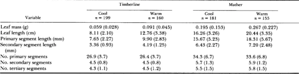
TABLE 1

Mean values and standard deviations (in parentheses) of leaf traits

Timberline Mather

Variable

Cool

n = 199

Warm

n = 160 n = 181

Cool

n = 155 Warm

Leaf mass (8) 0.059 (0.028) 0.091 (0.045) 0.195 (0.153) 0.267 (0.227) Leaf length (cm) 8.11 (2.10) 12.76 (3.38) 16.26 (3.26) 20.44 (3.35) Primary segment length (mm) _{7.65 (2.27)} _{9.90 (2.83)} _{15.67 (5.23)} _{18.31 (5.67)} Secondary segment length 3.36 (0.93) 4.19 (1.25) 6.43 (2.27) 7.20 (2.48)

No. primary segments 26.9 (3.7) 26.4 (3.7) 34.3 (6.7) 33.6 (6.8)

No. secondary segments _{4.5 (0.8)} _{4.5 (0.8)} _{5.7 (1.3)} _{5.9 (1.2)}

No. tertiary segments _{4.3 (1.1)} _{4.5 (1.2)} _{5.5 (1.5)} _{5.8 (1.5)}

(mm)

Means were calculated on log transformed data and then back-transformed. The standard deviations reported were calculated as the difference between the back-transformation of the mean plus one standard deviation and the back-transformed mean itself.

and appeared more open than Timberline leaves, and plants from both populations tended to produce larger and more open leaves in the warm bay than in the cool bay (Figure 1, Table 1 , and see below for statistical comparisons).

The differences in basic leaf shape among populations were not due to simple allometric scaling: that is, the leaves of the high altitude population were not merely scaled down versions of the larger leaves of the lower altitude population, but had different basic shapes. The relationship between leaf length and the length of the primary leaf segment was allometric (it was linear on a log scale, and not curvilinear) within populations in each growth environment. T h e slope of the regression of log leaf length on log primary segment length differed with growth environment and population (ANCOVA revealed a significant interaction between leaf length, population, and bay at

P = 0.05). Timberline plants had, on average, nar- rower leaves in proportion to their length (slope = 0.59, SE = 0.03, n = 358) than did Mather plants (slope = 0.74, SE = 0.07, n = 335). T h e allometric relationship (slope of the regression) between leaf length and primary segment length did not differ among growth environments for Timberline leaves; leaves in the warm environment were larger versions of those in the cool environment, with the same gross shape. Mather leaves responded differently to the two growth environments (P = 0.04), with leaf length increasing proportionately more than width in the warm environment (slope = 0.55, SE = 0.14, n = 154) as compared with the cool environment (slope = 0.89,

SE = 0.10, n = 180).

Achillea leaves were not obviously composed of self- similar units (Table 2). Leaves were relatively nar- rower than leaf segments (RATIO 1 was much smaller than RATIOP, both for untransformed and log transformed values (not shown)). T h e number of secondary segments was small relative to the number of primary segments, while the number of tertiary segments was

almost the same as the number of secondary segments (RATIO3 was much smaller than RATI04). These relationships were constant across populations and environments (not shown). This does not rule out the possibility that these leaves could be described using alternative measures of self-similarity, however (MAN- DELBROT 1983).

Canononical variate analysis: T h e canonical variate analysis showed strong separation between Mather and Timberline leaves, and less marked differences among warm and cool growth environments. T h e first two canonical variables (linear, multivariate combinations of the original measurements) were statistically significant (at P

<

0.0001), and accounted for 76% and 24% of the total variance in leaf measurements, respectively. Leaves with high values for the first canonical variable were larger (longer, and to a lesser extent, wider) than leaves with low values on the first axis. T h e factor that loaded most heavily on the first canonical variable was leaf length (the standardized canonical coefficient, SCC, was 0.77).

T h e length of the primary leaf segment also influ- enced the first canonical variable, but less strongly

(SCC = 0.33), while other variables had only small effects. As is common in CVA, the first canonical variable primarily summarizes size differences, while the second primarily contrasts shapes (REYMENT, BLACKITH and CAMPBELL 1984).

(5)

Leaf Shape Variation in Achillea

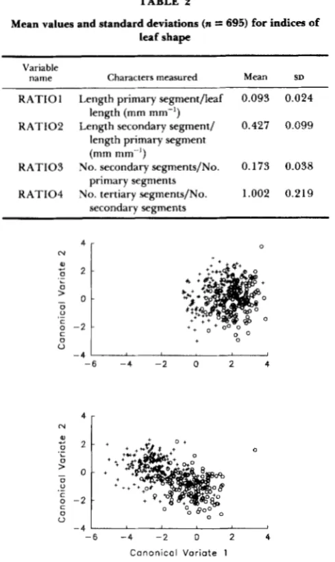
TABLE 2

Mean values and standard deviations (n

=

695) for indices of leaf shape

Variable

name Characters measured Mean SD

RATIO1 Length primary segment/leaf 0.093 0.024

RAT102 Length secondary segment/ 0.427 0.099 length (mm mm”)

length primary segment (mm mm”)

primary segments

secondary segments

RATIO3 No. secondary segments/No. 0.173 0.038

RATIO4 No. tertiary segments/No. 1.002 0.219

0

O - 4 I

-6 - 4 -2 0 2 4

- 6 - 4 - 2 0 2 4

Canonical V o r i o t e 1

FIGURE 2.-Canonical variate analysis. Each point represents the values for a single leaf from a Mather (top) or Timberline (bottom) plant on the first two canonical axes in the cool bay (+) and in the warm bay (0). Values for plants from the two populations are plotted separately for clarity of presentation.

packed with leaf segments, and those with low values were more loosely constructed. Differences in leaf shape as indicated by position on the second axis are independent of differences in leaf size.

Mather plants had high scores on the first canonical variable (Figure

2),

and Timberline had low scores, reflecting the larger size of Mather leaves. Timberline plants differed more than Mather plants among growth environments on that axis; that is, leaf size varied more with growth environment for Timberline than for Mather. Timberline had lower scores for the first canonical variable in the cool bay than in the warm bay (mean values were -2.4 in the cool bay and

-0.4 in the warm bay). Mather plants followed the same pattern, but were more closely clustered along CVA axis I (with means of 1.2 and 2.2 in the cool and warm bays, respectively). This is a result of the fact

TABLE 3

Mahalanobis squared distances between groups

Mather, Mather, Timberline, Timberline,

cool warm cool warm

Mather, cool

-

Mather, warm 1.53 -

Timberline, cool 13.20 21.77 -

Timberline, warm 4.87 7.82 5.56 -

that both populations produced larger leaves in the warm environment and smaller leaves in the cool environment. Both populations had higher values on the second canonical axis in the cool environment, and lower values in the warm environment (Figure

2).

This indicates that both populations produce leaves that were more tightly packed with segments, and shorter in relation to their width, in the cool environment. These are pure shape differences, with differences in leaf size effectively removed.

Examination of the Mahalanobis distances (Table 3) reinforces this picture. Mather leaves in the cool and warm environments were close to one another, while Timberline leaves differed in the two growth environments. Timberline leaves in the cool environment were very different from all Mather leaves, but Timberline leaves in the warm environment were similar to Mather leaves in the cool environment.

There was no substantive effect on the outcome of the canonical variate analysis of including those variables which were not normally distributed (secondary segment length, number of secondary segments, and number of tertiary segments); these factors played little part in defining differences in shape within and among populations and growth environments. Results reported are for analyses with those variables omitted. High correlations among characters may affect the outcome of CVA (MANLY 1986). Correlations (within populations) between the log transformed variables were generally moderate and positive, ranging from

ca. 0.2 to 0.7, with most values below 0.5. Thus the correlations among variables should not distort the results of the multivariate analysis to any substantial degree.

(6)

390 J. Gurevitch

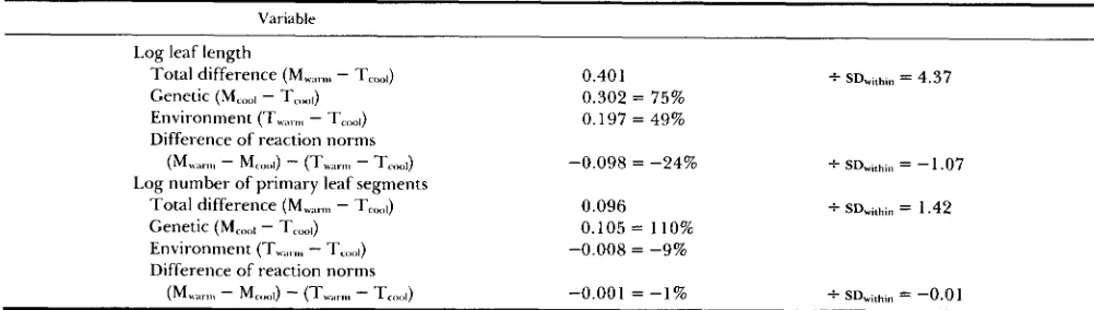
TABLE 4

Causes of differences in mean phenotypes

Variable

Log leaf length

Total difference (M,;,,,,, - T,,,,) 0.401 f SD,,lh,n = 4.37

Genetic (M,,,,,I - T,,,,,I) 0.302 = 75%

Environment (T,,,,,, - T,,,,I) 0.197 = 49% Difference of reaction norms

(M,.,,,,, - M,,,,,I)

-

(Tx.3rm,l - T,,,,I) -0.098 = -24% f SD,,thi,, = -1.07 Log number of primary leaf segments

Total difference (M,.,,,,, - T,,,,,,) 0.096 f SD,ithin = 1.42 Genetic (M,,,,,I - T<,,I) 0.105 = 110%

Environment (T,.,,,,,

-

T,,,,,I) -0.008 = -9% Difference of reaction norms

(M,;,,,,, - M<<,,,I)

-

(T,.,,,,,

-

T,,,,,I) -0.001 = - 1 % f SD,;,hln = -0.01

Abbreviations: M , Mather population; T, Timberline population; SD, within-population (phenotypic) standard deviation.

per leaf was analyzed with and without leaf length as a covariate to contrast differences in the absolute number of segments with differences in how tightly segments were packed.

Leaf length differed strongly among populations (Tables 1 and 4, F = 290.6, d.f. = 1,50.5, P

<

0.0001) and among growth environments ( F = 225.9, d.f. = 1, 10.8, P

<

0.0001). T h e populations responded differently to growth environments, with Timberline leaves increasing more steeply in length in response to the warm environment than did Mather leaves (Table 1; the interaction between population and growth environment for leaf length was significant, with F = 53.2, d.f. = 1, 639, P

<

0.0001). There were

also genetic differences in leaf length within populations (for genets nested within populations, F = 6.2, d.f. = 47, 639, P

<

O.OOOl), and differences in leaf length due to the block in which a plant was located (for blocks nested within bays, F = 2.5, d.f. = 10, 639, P = 0.0056).

If Mather leaves in their natural environment are approximated by those in the warm bay, and Timber- line leaves by those in the cool bay, we can examine the causes of the differences between the populations and the relative importance of genetic (referring here to genetic differences between populations) and environmental causes (Table 4). T h e genetic (ie., population) difference is larger than that caused by the environment, but both are substantial. T h e difference of Mather and Timberline reaction norms is also substantial, but is in the opposite direction (ie., it is negative). The total difference and the difference of reaction norms are also substantial when scaled by the within-population phenotypic standard deviation.

Because the two populations responded to growth environment differently, variation was also analyzed separately for Mather and Timberline. For the Tim- berline plants, leaf length was greater in the warm environment ( F = 159.5, d.f. = 1, 14.5, P

<

0.0001)

and also differed among blocks ( F = 1.9, d.f. = 10, 184.9, P = 0.045). There was genetic variation within the Timberline population in leaf length ( F = 4.4, d.f. = 23, 22.5, P = 0.0004). Genotype-environment interactions were not significant for the Timberline plants. T h e length of Mather leaves was also greater in the warm environment ( F = 80.2, d.f. = 1, 17.5, P

<

O.OOOl), but did not vary among blocks within bays (F=1.5,d.f.=10,177.7,P=0.2).Therewasgenetic variation within the Mather population in leaf length

( F = 3.4, d.f. = 24, 23.6, P = 0.002), and there was a significant interaction between genotypes and growth environments ( F = 1.7, d.f. = 24, 187.7, P = 0.024). T h e number of primary segments per leaf was substantially greater for Mather than for Timberline leaves (Tables 1, 4, F = 67.8, d.f. = 1, 50.6, P

<

0.0001). There were genetic differences in this trait within populations ( F = 6.0, d.f. = 47, 47, P

<

O.OOOl), and differences in the responses of genets to growth environment (the effect of genets nested within populations X bay was significant at F = 1.6, d.f. = 47, 587, P = 0.008). The growth environment did not directly affect the number of segments ( F =

1.9, d.f. = 1, 28.2, P = 0.18), nor was there any difference between populations in the response to growth environment (the population X bay interaction was not significant, with F = 0.09, d.f. = 1, 70.2, P = 0.76).

(7)

Leaf Shape Variation in Achillea 391

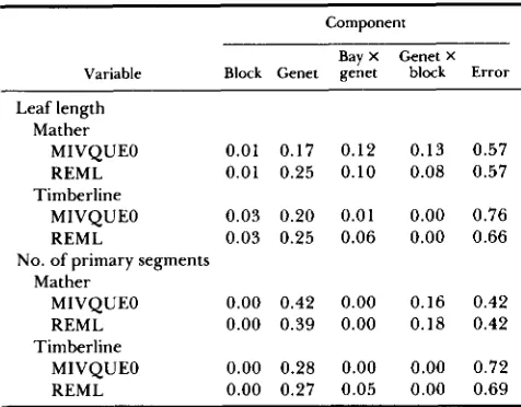
TABLE 5

Components of variance for two leaf traits

Component

Variable Block Genet genet block Error Bay X Genet X

Leaf length Mather

MIVQUEO 0.01 0.17 0.12 REML 0.01 0.25 0.10

MIVQUEO 0.03 0.20 0.01 REML 0.03 0.25 0.06 Timberline

No. of primary segments Mather

MIVQUEO 0.00 0.42 0.00 REML 0.00 0.39 0.00

MIVQUEO 0.00 0.28 0.00 REML 0.00 0.27 0.05 Timberline

0.13 0.08

0.00 0.00

0.16 0.18

0.00 0.00

0.57 0.57

0.76 0.66

0.42 0.42

0.72 0.69

Proportions of variance calculated by minimum variance quadratic unbiased estimator (MIVQUEO) and restricted maximum likelihood (REML) methods.

The degree to which segments are packed in along the length of the leaf can be examined by analyzing the number of primary segments per leaf with leaf length as a covariate. This essentially holds leaf length constant, focusing on the residual variation in the number of segments. Leaf length as a covariate had a highly significant effect on the number of segments

( F = 3 1.1, d.f. = 1, 586, P

<

0.0001). With leaf length as a covariate, the number of primary segments differed significantly (at P

<

0.0005) among populations, growth environments, and genets, and there were significant effects ( P = 0.001) of the interactions between genets and growth environments. T h e effect of blocks, and the interaction between populations and growth environments were not significant.

Components of variance: leaf length and number of primary segments: Within each population, the magnitude of the genetic determination of leaf length was moderate (broad-sense heritability was approximately 0.2; Table 5). Heritability for the number of primary segments was somewhat greater (approximately 0.3 for Timberline and 0.4 for Mather; Table

5 ) . The small-scale within-environment effects of blocks did not account for any of the variation among individuals in either population for either measure of leaf shape. However, Mather plants had measurable interactions between genotype and environment at both the large scale (genet X bay) and small scale (genet X block (bay)) for leaf length, and on the small scale for number of primary segments (Table 5). Tim- berline did not exhibit these interactions. When

growth environment ( L e . , bay) was included in the model as if it were a random variable, it accounted for 48% of the total variance in leaf length for Mather and 65% for Timberline (in addition to the total

TABLE 6

Components of variance within populations for canonical variates 1 and 2

Component

Bay X Genet X

Variates Block Genet genet block Error

Canonical variate 1

Mather

MIVQUEO 0.00 0.17 0.06 0.21 0.56 REML 0.00 0.24 0.05 0.14 0.56 Timberline

MIVQUEO 0.02 0.23 0.01 0.00 0.75 REML 0.03 0.30 0.03 0.01 0.64 Canonical variate 2

Mather

MIVQUEO 0.00 0.26 0.02 0.06 0.66 REML 0.00 0.29 0.05 0.06 0.60 Timberline

MIVQUEO 0.01 0.06 0.15 0.00 0.79 REML 0.01 0.04 0.18 0.00 0.76 Proportions of variance calculated by minimum variance quadratic unbiased estimator (MIVQUEO) and restricted maximum likelihood (REML) methods.

variance accounted for by the true random factors). In both populations growth environment accounted for none (0%) of the variance in the number of primary segments. A substantial proportion of the total variance was not accounted for by the environmental and genetic factors included in the model (Table 5). Estimates of the variance components based on the MIVQUEO and REML methods agreed well, suggesting that the estimates are robust to the structure of the data.

Variation within populations in canonical var- iates 1 and 2: Variation within populations in leaf size and shape is summarized by the multivariate scores for canonical variates one and two. Canonical variate one primarily summarizes size differences, while the second canonical variate is a reflection of overall shape differences among plants (see above). Mather plants had moderate broad sense heritabilities for both size and shape as represented by the first and second canonical variates (Table 6 ) . There was also a substantial variance component for the genet X environment (genet X block) interaction for size. Other terms ex- plained by the model were small or zero for both variates for Mather. T h e Timberline population also displayed moderate heritability for the first variate, but heritability for leaf shape (variate two) was small. T h e proportion of variance for other factors was small in the Timberline plants, except for a moderate norm of reaction (bay X genet) value for leaf shape.

DISCUSSION AND CONCLUSIONS

(8)

392 J. Gurevitch

mative responses of leaf morphology to temperature (additional factors may also affect Achillea leaf morphology in the field). T h e genetic differentiation between the high and low altitude populations parallels the plastic response to growth temperature. At high altitudes, leaves are shorter and more fully packed with segments, while at lower altitudes leaves are longer and more open. When grown in a common environment, plants of a high and a lower altitude population retained these differences in leaf size and shape. In a cool growth environment, both populations produced leaves that likewise were shorter and more fully packed with leaf segments, while in a warm environment leaves of both populations were longer and more loosely filled with segments, resulting in a more open structure. T h e Mahalanobis distances in the CVA further support this picture, demonstrating that Timberline leaves in the cool environment were most different from Mather leaves in the warm environment, while Timberline leaves in the warm environment were much closer to Mather leaves in the cool environment. T h e agreement between plastic and genetic alteration in leaf shape suggests that the contrasting morphologies may provide adaptive ad- vantages in each environment (GUREVITCH 1988; GUREVITCH and SCHUEPP 1990).

Other authors have also reported genetic differences among populations of herbaceous plants in leaf length (or other simple measures of leaf size) with smaller leaves at higher altitudes, and with lower altitude populations and warmer growth environments producing relatively longer or larger leaves (e.g., CLAUSEN, KECK and HIESEY 1940, 1948; HIESEY

1953; MOONEY and BILLINGS 196 1 ; SHAVER, FETCHER and CHAPIN 1986; WOODWARD 1983; WOODWARD, KORNER and CRABTREE 1986; KORNER et al. 1989; and see BILLINGS and MOONEY 1968). Many of these experimental studies also report considerable plastic- ity in plant size with respect to growth environment. Results of the present study are generally consistent with previous findings.

While variation within plant populations in simple measures of size, such as leaf length and width, has been examined experimentally, comparisons of leaf shape are more commonly made for material collected in the wild, with the aim of using morphological differences to distinguish taxa (see DICKINSON, PAR-

KER and STRAUSS 1987 for a review of quantitative leaf shape comparisons). Because the material collected typically comes from different taxa in different environments, it is not possible to separate genetic and plastic sources of variation in leaf shape in such studies (but see HELGADOTTIR and SNAYDON 1986).

Modern morphometric techniques are considerably more developed for describing the shapes of animals than plants (ARTHUR 1984; REYMENT, BLACKITH and

CAMPBELL 1984) (and see ATCHLEY, RUTLEDGE and COWLEY 198 1 ; DICKINSON, PARKER and STRAUSS 1987). Even for animals, the vast majority of morphometric studies have been descriptive and not experimental (ATCHLEY, RUTLEDGE and COWLEY 1981); systematic in purpose rather than focusing on genetic problems. Botanists have historically tended to rely upon verbal descriptions of leaf shape characters, or on highly simplified measurements of shape. Less frequently, workers have attempted to quantify lobed or complex leaf shapes. In a noteworthy example, LEWIS (1969) found genetic differentiation in leaf dissection in Geranium sanguineum, with more dissected leaves being associated with dry, continental habitats. T h e adaptive significance of variation in leaf size and shape in G . sanguineum was interpreted in terms of the energy budgets and consequent temperatures of leaves of different shape (LEWIS 1972). Other examples of quantification of complex leaf shapes include MCLELLAN’s (1990) work on the de- velopmental basis of differences in lobing and the depth of incision among varieties of Begonia dregei, and the use of multivariate analyses of lobed leaves in the identification of species, varieties, and hybrids in red oaks (HICKS and BURCH 1977; JENSEN 1989). Often those attempting to quantify leaf shape suc- cumb to the temptation to describe shape in terms of ratios (leaf length to leaf width, leaf area to leaf mass, lobe length to sinus depth, and so on). These ratios are fraught with problems in analysis and interpreta- tion, and multivariate and other approaches are to be strongly preferred (ATCHLEY, GASKINS and ANDER-

SON 1976; DICKINSON, PARKER and STRAUSS 1987;

BOOKSTEIN 1978; REYMENT, BLACKITH and CAMP-

BELL 1984).

Heritabilities for leaf size and shape variables in the present study were generally substantial. While the estimates for the heritability of leaf length agreed well with previous reports for heritabilities for leaf size characters in wild plants (e.g., ANTLFINGER 198 1 ; SIL-

ANDER 1985; SCHEINER, GUREVITCH and TEERI 1984;

SHAVER et al. 1986), there are no comparable figures published that I am aware of for leaf shape characters as distinguished from leaf size.

(9)

justment. Here, however, there was no apparent trade-off between genetic control over morphology and the capacity for directional (as contrasted with random) plastic response to the environment. Plastic change in Timberline leaves in response to the temperature of the growth environment was allometric, but Mather leaves were of different basic shapes in the warm and cool environments. T h e implications of this contrast remain to be explored in future work.

It is intriguing that the shape of these complex leaves is not created merely by an elaboration of the same structure at different scales (i.e., self-similarity). This suggests that leaf shape is under strict develop- mental and genetic control and may be adaptive. If natural selection is acting merely to alter leaf size at different altitudes, one would expect that shape differences among populations would be allometric. That was not the case: Timberline leaves differed from Mather leaves in both size and shape, and shape did not differ in a simple allometric fashion between populations. This, too, suggests that selection has acted specifically on leaf shape in each habitat, and that the contrasting shapes may be adaptive in the different thermal environments at low and high altitudes.

1 gratefully acknowledge the generosity of Professor F.A. BAZZAZ of Harvard University, in whose lab this work was conducted, and support by a Katherine Putnam Fellowship at The Arnold Arbor- etum of Harvard University. TODD POSTOL, MONICA HEXNER, DIANE HERBERT, MIAO SHILI, JANET MORRISON, CONRAD SMITH a nd PAUL TEESE provided critical logistical support in handling hundreds of plants and in making thousands of measurements. DON BUCKLEY and RICHARD PRIMACK offered suggestions, help and discussion which were much appreciated. This is contribution 805 in Ecology and Evolution at the State University of New York at Stony Brook.

LITERATURE CITED

ANTLFINGER, A. E., 1981 T h e genetic basis of microdifferentia- tion in natural and experimental populations of Borrichia fru- tescens in relation to salinity. Evolution 35: 1056-1068. ARGYRES, A. Z., and J. SCHMITT, 1991 Microgeographic genetic

strudture of morphological and life history traits in a natural population of Impatiens capensis. Evolution 45: 178-1 89. ARTHUR, W., 1984 Mechanisms of Morphological Evolution. John

Wiley & Sons, Chichester.

ATCHLEY, W. R., C. T. GASKINS and D. ANDERSON, 1976 Statistical properties of ratios. I . Empirical results. Syst. Zool. 25: 137-148.

ATCHLEY,

w.

R.,J. J. RUTLEDGEand D. E. COWLEY, 1981 Genetic components of size and shape. 11. Multivariate covariance patterns in the rat and mouse skull. Evolution 35: 1037-1055, BALDING, F. R., and G. L. CUNNINGHAM, 1976 A comparison of

heat transfer characteristics of simple and pinnate leaf models. Bot. Gaz. 137: 65-74.

BILLINGS, W. D., and H. A. MOONEY, 1968 T h e ecology of arctic and alpine plants. Biol. Rev. 43: 481-529.

BOOKSTEIN, F. L., 1978 The Measurement of Biologrcal Shape and Shape Change (Lecture Notes in Biomathematics, 24). Springer- Verlag, Berlin.

CAMPBELL, G. S., 1977 An Introduction to Environmental Biophysics. Springer-Verlag, New York.

CLAUSEN, J., D. D. KECK and W. M. HIESEY, 1940 Experimental Studies on the Nature of Species. I. Effect of Varied Environments on Western North American Plants. Carnegie Inst. Wash. Publ. 520.

CLAUSEN, J., D. D. KECK and W. M. HIESEY, 1948 Experimental Studies on the Nature of Species. 111. Environmental Responses of Climatic Races of Achillea. Carnegie lnst. Wash. Publ. 581. DICKINSON, T . A , , W. H . PARKER AND R. E. STRAUSS,

1987 Another approach to leaf shape comparisons. Taxon

36: 1-20.

FALCONER, D. S., 1981 Introduction to Quantitative Genetics, Ed. 2. Longman, New York.

GATES, D. M., 1980 Biophysical Ecology. Springer-Verlag, N. Y. GIVNISH, T . , 1979 On the adaptive significance of leaf form, pp.

375-407 in Topics in Plant Population Biology, edited by 0. T.

SOLBRIG, S. JAIN, G. B. JOHNSON and P. H. RAVEN. Columbia University Press, New York.

GUREVITCH, J., 1988 Variation in leaf dissection and leaf energy budgets among populations of Achillea from an altitudinal gradient. Am. J. Bot. 75: 1298-1306.

GUREVITCH, J., and P. H. SCHUEPP, 1990 Boundary layer properties of highly dissected leaves: an investigation using an electrochemical fluid tunnel. Plant Cell Environ. 13: 783-792. HARTLEY, H. O., J. N. K. RAO and L. LAMOTTE, 1978 A simple

synthesis-based method of variance component estimation. Bio- metrics 3 4 233-242.

HELGADOTTIR, A., and R. W. SNAYDON, 1986 Patterns of genetic variation among populations of Poa pratensis L. and Agrostis capillaris L. from Britain and Iceland. J. Appl. Ecol. 23: 703- 719.

HICKS, R. R., and J. B. BURCH, 1977 Numerical taxonomy of southern red oak in the vicinity of Nacogdoches, Texas. For. Sci. 23: 290-298.

HIESEY, W. M., 1953 Comparative growth between and within climatic races ofAchillea under controlled conditions. Evolution

JENSEN, R. J., 1989 T h e Quercus falcata Michx. complex in Land Between the Lakes, Kentucky and Tennessee: a study of mor- phological variation. Am. Midl. Nat. 121: 245-255.

KORNER, C., and M. DIEMER, 1987 In situ photosynthetic responses to light, temperature and carbon dioxide in herbaceous plants from low and high altitude. Funct. Ecol. 1: 179-194.

KORNER, C., M. NEUMAYER, S. P. MENENDEZ-RIEDL and A. SMEETS- SCHEEL, 1989 Functional morphology of mountain plants. Flora 182: 353-383.

LEWIS, M. C., 1969 Genecological differentiation of leaf morphology in Geranium sanguinium L. New Phytol. 68: 481-503. LEWIS, M. C., 1972 T h e physiological significance of variation in

leaf structure. Sci. Progr. Oxford 60: 25-51.

MANDELBROT, B. B., 1983 The Fractal Geometry of Nature. W. H. Freeman, New York.

MANLY, B. F. J., 1986 Multivariate Statistical Methods: A Primer. Chapman & Hall, London.

MANLY, B. F. J., 1991 Randomization and Monte-Carlo Methods in Biology. Chapman & Hall, London.

MCLELLAN, T . , 1990 Development of differences in leaf shape in Begonia dregei (Begoniaceae). Am. J. Bot. 77: 323-337. MILLIKEN, G. A . , and D. E. JOHNSON, 1984 Analysis of Messy Data.

Volume 1: Designed Experiments. Lifetime Learning Pubs. (Wads- worth, Inc.), Belmont, Calif.

MOONEY, H . A., and W. D. BILLINGS, 1961 Comparative physiological ecology of arctic and alpine populations of Oxyria digyna. Ecol. Monogr. 31: 1-29.

ORIANS, G. H., and 0. T . SOLBRIG, 1977 A cost-income model of leaves and roots with special reference to arid and semi-arid areas. Am. Nat. 111: 667-690.

PARKHURST, D. F., and D. L. LOUCKS, 1972 Optimal leaf size in relation to environment. J. Ecol. 60: 5505-5537.

(10)

394 J.

KASCHKE, K., 1960 Heat transfer between the plant and the environment. Annu. Rev. Plant Physiol. 11: 11 1-126.

KEYMENT, R. A,, R. E. BLACKITH and N. A. CAMPBELL, 1984 Multivariate Morphometrics, Ed. 2. Academic Press, Lon- don.

SAS Institute, 1988 SASISTAT User’s Guide. SAS Institute, Cary, N.C.

SCHEINER, S . M., J. GUREVITCH and J. A. TEERI, 1984 A genetic analysis of the photosynthetic properties of populations of Danthonia spicata that have different growth responses to light level. Oecologia 64: 74-77.

SHAVER, G. R., N. FETCHER and F. S. CHAPIN 111, 1986 Growth and flowering in Eriophorum vagznatum: annual and latitudinal variation. Ecology 67: 1524-1535.

SILANDER, J. A. JR., 1985 The genetic basis of the ecological amplitude of Spartina patens. 11. Variance and correlation analysis. Evolution 39: 1034-1052.

SLATYER, R. O., and P. J. FERRAR, 1977 Altitudinal variation in the photosynthetic charracteristics of snow gum, Eucalyptus pauczflora Sieb. ex Spreng. 11. Effects of growth temperature

under controlled conditions. Aust. J. Plant Physiol. 4: 289- 299.

SMITH, W. K., and P. S. NOBEL, 1978 The influence of leaf temperature, soil water potential, and illuminaiton on leaf morphology in Encelia farinosa Gray. Am. J. Bot. 28: 171-185. TAYLOR, S. E., 1975 Optimal leaf form, pp. 213-238 in Perspec-

tives of Biophysical Ecology, edited by P. M. GATFS and R. B. SCHMERL. Springer-Verlag, New York.

TURESSON, G., 1922 The genotypical response of the plant species to the habitat. Hereditas 3: 21 1-350.

TURESSON, G., 1925 The plant species in relation to habitat and climate. Contributions to the knowledge of genecological units. Hereditas 6: 147-236.

VOGEL, S., 1970 Convective cooling at low airspeeds and the shapes of broad leaves. J. Exp. Bot. 21: 91-101.

WILLIAMS, B. K., 1983 Some observations on the use of discriminant analysis in ecology. Ecology 6 4 1283- 129 1.

WOODWARD, F. I . , 1983 The significance of interspecific differences in specific leaf area to the growth of selected herbaceous species from different latitudes. New Phytol. 95: 313-323. WOODWARD, F. I., C . KORNER and R. C. CRABTREE, 1986 The

dynamics of leaf extension in plants with diverse altitudinal ranges. Oecologia 7 0 222-226.