ABSTRACT
BUCCI, MICHAEL JAMES. Solution Procedures for Logistics Network Models with Economies of Scale. (Under the direction of Michael G. Kay and Donald P. Warsing.)
As supply chains have become more dynamic the difference in the time horizon for strategic
decisions has diminished, resulting in supply chains that are more flexible with no/low fixed
facility costs. This trend requires the development of solution approaches that can combine
the traditionally separate strategic, tactical, and operational decisions in an integrative
manner, incorporating a range of decision variables and cost considerations while producing
good, and possibly near-optimal, solutions in reasonable time.
This research begins to address these issues through the development of heuristic
approaches to solve large-scale facility location problems that reflect economies of scale in
the per-unit costs of processing goods and/or holding safety stock of those goods to protect
against uncertainty in demand. Such non-linear economies of scale are well known in
practice, but are often excluded or overly simplified in location models due to their
non-linear nature. Combining and extending existing heuristic approaches, we develop and
analyze several meta-heuristics to solve a location problem with a non-linear, concave cost
function, which is used as a surrogate for more computationally complex cost functions.
The resulting solution methods offer near-optimal solutions with relatively modest
computational effort. These meta-heuristics are then applied to a focused study on the use
of approximations to represent safety stock inventory costs in location models. This
research evaluates the commonly used ―Square Root Law‖ and a more general concave cost
function against the explicit safety stock inventory calculation in models with and without
inter-customer demand correlation. The results highlight the conditions for which these
functions accurately approximate actual inventory costs and/or when they generate location
solutions that are close to those generated by the explicit computation of inventory levels.
industry. This application requires us to recommend locations for processing used carpet in
a setting where the recycling facilities to be located exhibit economies of scale in
processing. We use our modeling approach to analyze an existing, smaller-scale used carpet
collection network and also evaluate a larger hypothetical national collection network,
providing insight into the number of recycling facilities that should be located and their
respective size. We compare the results of formulating and solving models with and without
Solution Procedures for Logistic Network Design Models with Economies of Scale
by
Michael James Bucci
A dissertation submitted to the Graduate Faculty of North Carolina State University
in partial fulfillment of the requirements for the degree of
Doctor of Philosophy
Industrial Engineering
Raleigh, North Carolina
2009
APPROVED BY:
_______________________________ ______________________________
Michael G. Kay Donald P. Warsing
Committee Co-Chair Committee Co-Chair
_______________________________ ______________________________
ii BIOGRAPHY
Michael J. Bucci was born in Endicott, NY. He graduated from Union-Endicott High
School in 1986, and then obtained an undergraduate degree in Ceramic Engineering at
Alfred University in 1990. Mike then worked for one year before returning to study for his
master‘s degree in Industrial Engineering at Binghamton University (SUNY) under the
supervision of Dr. R.E. Emerson. From here, Mike worked in industry for nine years in a
variety of engineering and management positions. He then returned to academia to pursue a
degree in Industrial and Systems Engineering at North Carolina State University under the
supervision of Dr. Michael Kay and Dr. Donald Warsing. Mike and his wife are the proud
iii ACKNOWLEDGEMENTS
I would like to thank the following people for their generous and continued support for this
work:
Dr. Michael Kay and Dr. Donald Warsing served as my advisors and co-chairs. Both
provided invaluable support and guidance to me throughout this journey.
Dr. Reha Uzsoy and Dr. Jeffrey Joines served as my committee members, and I
iv TABLE OF CONTENTS
LIST OF TABLES ... vi
LIST OF FIGURES ... vii
CHAPTER 1: Introduction ... 1
Introduction ... 1
Dissertation Outline ... 1
Overview of Chapters ... 1
CHAPTER 2: Metaheuristics for Facility Location Problems with Economies of Scale ... 4
Abstract ... 5
1. Introduction ... 5
2. Literature Review ... 6
3 Model Formulation ... 9
4. Computational Results ... 10
4.1 Experimental Design ... 10
4.2 Metaheuristic Solution Approaches for Smaller Problems ... 12
4.3. Performance of Metaheuristics on Smaller Problems ... 20
4.4 Metaheuristic Solution Approaches for Larger Problems ... 24
4.5 Performance of Metaheuristics on Larger Problems ... 24
5. Conclusions and Directions for Future Work ... 27
6. Acknowledgments ... 28
7. References ... 28
CHAPTER 3: Modeling Inventory Pooling Effects in Facility Location ... 31
Abstract ... 32
1. Introduction ... 32
2. Literature Review ... 34
3. Model Formulation ... 38
4. Computational Results ... 40
4.1 Experimental Design ... 40
4.2 Metaheuristic Solution Approach ... 44
4.3. Results from Model without Correlation ... 45
4.4 Results from Models with Correlation ... 53
5. Conclusions and Directions for Future Work ... 55
6. Appendix 3A: Procedure for Generating Valid Correlation Matrices ... 56
7. References ... 60
CHAPTER 4: An Application of Heuristics Incorporating Economies of Scale to Facility Location Problems in Carpet Recycling ... 63
Abstract ... 64
1. Introduction ... 64
2. Relevant Research ... 65
v
3. Case Study ... 69
3.1 Results... 72
4. Conclusions and Directions for Future Work ... 77
5. Acknowledgments ... 78
6. References ... 78
CHAPTER 5: Conclusions and Directions for Future Work ... 80
5.1 Conclusions... 80
5.2. Future Work ... 81
APPENDICES ... 83
Appendix A: Supplemental Information for Chapter 2 ... 84
A.1.0 Reprint of Journal Paper: IERC 2006 ... 84
A.1.1 Reprint of Journal Paper: IERC 2007 ... 96
A.1.2 Additional data not included in journal paper ... 110
A.1.3 MATLAB code ... 115
Appendix B: Supplemental Information for Chapter 3 ... 178
B.1.1 MATLAB code ... 178
Appendix C: Supplemental Information for Chapter 4 ... 217
C.1.0 Additional data not included in journal paper ... 217
vi LIST OF TABLES
Chapter 2:
Table 1: Metaheuristics Analyzed on Smaller Instances ... 13
Table 2: Comparison of Average Total Cost and Average Solution Time... 21
Table 3: Comparison of the Average Number of Evaluations using xFB Measurement ... 22
Table 4: Heuristics Analyzed on Larger Instances ... 24
Table 5: Comparison of Average Total Cost and Average Solution Time... 25
Table 6: Comparison of the Average Number of Evaluations using xFB Measurement ... 26
Chapter 3: Table 1: Inventory Cost Analysis for Independent Demand Case ... 48
Table 2: Average Facility Size for the Five Largest Facilities in each Experiment ... 50
Table 3: Impact of Parameter Values on the accuracy of SRL1 and SRL2 ... 51
Table 4: Average Total Cost and Solution Structure Values ... 53
Table 5: Average values from Inter-customer Correlation experiments ... 55
Chapter 4: Table 1: Summary of Recommended Solution for each Model Studied ... 77
Appendix A.1.0 Table 1: Supply Chain Parameters ... 88
Table 2: Run 1, largest facility percentage for lowest cost solution ... 91
Table 3: Run 1, percentage of repetitions within 5% of the best run ... 91
Table 4: Run 2, largest facility weight for lowest cost solution ... 92
Table 5: Run 2, percentage of repetitions within 5% of the best run ... 92
Appendix A.1.1 Table 1: Summary of Heuristic Analyzed ... 101
Table 2: Results—Comparison of Heuristics ... 103
Table 3: Comparison of the percent reduction in computational evaluations ... 105
Appendix B Table 1 Characteristics of ―W‖ heuristics ... 110
vii LIST OF FIGURES
Chapter 2:
Figure 1: Solution Procedure for W1 Heuristic ... 16
Figure 2: Example of a re-location set for the W1 and W2 Heuristics ... 17
Figure 3: Example of a re-allocation set for the W1 and W1-LAt Heuristics ... 18
Figure 4: Example of construction subset for n = 200 and ms = 50 ... 19
Chapter 3: Figure 1: Partitioning of the Solution Space for the Creation of the Correlation Matrix ... 43
Figure 2: General Solution Procedure for W2-S-Lat Heuristic (Bucci et al. 2009) ... 45
Figure 3: Inventory Difference between SRL0 and SRL1 and SRL2 for all twenty four experiments ... 49
Figure 4: Average Size of Facilities for a subset of the Experiments (facilities sizes sorted largest to smallest) ... 49
Figure 5: Inventory Level Requirements as the Number of Facilities in the Solution Increases ... 54
Chapter 4: Figure 1: CARE Reclamation Network – [CARE 2009] ... 67
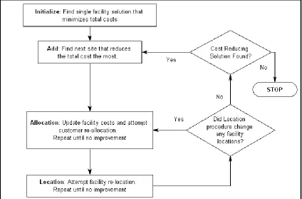
Figure 2: General Flow of the Solution Meta-heuristic [Bucci et al. 2009] ... 68
Figure 3: Recycling Center Processing Costs as a Function of Facility Size ... 71
Figure 4: Collection Center Locations for 400 Customer model ... 72
Figure 5: CARE network solution with no economies of scale in processing costs ... 73
Figure 6: CARE network solution with economies of scale in processing costs ... 73
Figure 7: 400-customer solution with 300M lb of demand, and economies of scale in processing costs ... 74
Figure 8: 400-customer solution with 600M lb of demand, and economies of scale in processing costs ... 74
Figure 9: 400-customer solution with 1200M lb of demand, and economies of scale in processing costs ... 75
Figure 10: 400-customer solution with 1800M lb of demand, and economies of scale in processing costs ... 75
Figure 11: 400-customer solution with 2400M lb of demand, and economies of scale in processing costs ... 76
Figure 12: 400-customer solution with 1800M lb of demand, and no economies of scale in processing costs ... 76
Appenix A.1.1 Figure 1: Example of an initial facility location-allocation ... 89
Figure 2: Example of intermediate facility location-allocation ... 89
viii Appendix A.1.2
1 CHAPTER 1: Introduction
Introduction
As supply chains have become more dynamic the difference in the time horizon for strategic
decisions has diminished, resulting in more flexible supply chains with no/low fixed facility
costs. This trend necessitates the development of solution approaches that can evaluate the
traditionally separate strategic, tactical, and operational decisions in an integrative manner,
incorporating a range of decision variables and cost considerations while producing good,
and possibly near-optimal, solutions in reasonable time. This research studies these types of
facility location allocation problems by extending traditional facility location models and
their associated solution techniques. The solution methods envisioned for these types of
models combine multiple techniques such as metaheuristics, simulation, and optimization
methods into a flexible framework to solve problems of realistic practical size.
Dissertation Outline
Chapters 2, 3, and 4 are structured as self-standing journal submissions. Each of these
chapters is formatted to the requirements of the journal for which they were submitted or are
intended to be submitted. Chapter 5 provides conclusions and directions for future work for
the entire dissertation. The Appendices include supplemental information for chapters two,
three, and four that were not suitable to include in the journal publications. This includes
original data, computer programs, and additional observations and findings. Additionally,
two short conference paper submissions are given in Appendix A. These papers were a
precursor to the more detailed journal paper displayed in Chapter 2.
Overview of Chapters
Chapter 2 investigates facility location models that incorporate economies of scale in unit
costs of production and/or inventory holding. These models have known customer locations
2 distribution centers to minimize transportation costs and facility costs, the latter being
composed of fixed costs and variable costs that are non-linear in the number of units
processed. To solve these models several metaheuristic solution approaches were developed
by combining and extending existing techniques. These solution approaches were compared
in an extensive empirical study with the results, highlighting the combinations of techniques
that can find near-optimal solutions with moderate computational effort. Since our objective
is to assess the ability to solve problems with objective functions that are more complex to
calculate, new measures of computational effort are developed.
Chapter 3 investigates methods for modeling risk-pooling effects associated with
centralizing safety stocks in large-scale facility location models. These models have known
customer locations with stochastic demands, and the objective is to locate an unknown
number of distribution centers to minimize the transportation and safety inventory costs.
The ―Square Root Law‖ and a more general concave cost function, which accounts for
facility size more explicitly, are compared with the explicit calculation of safety stock
inventory on the basis of total solution cost, solution time, and solution structure. Models
with no correlation in demand across customer locations are studied along with models that
include inter-customer demand correlation. The latter effort also resulted in a new method
for generating large scale matrices for inter-customer correlation in demand. The results
from models with no inter-customer correlation of demand show that the ―Square Root
Law‖ is fairly inaccurate at estimating inventory costs due to the assumptions underlying this rule, while the more general concave cost function always outperforms the ―Square Root Law‖ with minimal additional computational effort. In models with low and moderate
inter-customer correlation of demand, both approximation techniques poorly estimate the
inventory required, suggesting the need to use the explicit calculation or the development of
3 Chapter 4 investigates an industry application: a reverse logistics network for recycling used
carpet. The model attempts to minimize the total cost to locate an unknown number of
carpet recycling facilities that process used carpet collected from an established network of
collection points. The model includes transportation cost from the collection facility to the
recycling facility, fixed facility costs at the recycling facility, and non-linear processing
costs at the recycling facility, the latter exhibiting economies of scale as the facility size
increases. The model evaluates a known carpet collection network and a hypothetical
collection network that assumes a significant increase in collection locations and collection
rates to meet carpet industry recycling targets. We show that economies of scale have a
significant impact on the solution structure, and also demonstrate the impact that collection
4 CHAPTER 2: Metaheuristics for Facility Location Problems with Economies of Scale
Michael J. Bucci*, Michael G. Kay*, Donald P. Warsing†,Jeffrey A. Joines**
*Fitts Department of Industrial and Systems Engineering, North Carolina State University, Raleigh, NC 27695, USA †
Department of Business Management, North Carolina State University, Raleigh, NC 27695, USA **Department of Textile Engineering/Chemistry/Science, North Carolina State University, Raleigh, NC 27695, USA
5
Metaheuristics for Facility Location
Problems with Economies of Scale
Michael J. Bucci*, Michael G. Kay*, Donald P. Warsing†,Jeffrey A. Joines**
*Fitts Department of Industrial and Systems Engineering, North Carolina State University, Raleigh, NC 27695, USA †
Department of Business Management, North Carolina State University, Raleigh, NC 27695, USA **
Department of Textile Engineering/Chemistry/Science, North Carolina State University, Raleigh, NC 27695, USA
Abstract
We develop solution methods for solving large-scale facility location problems that include non-linear costs, reflecting economies of scale in unit costs of production and/or safety stock inventory. Through an extensive empirical study we compare several metaheuristic solution methods that combine algorithmic construction, allocation, and location techniques,
including alternate location-allocation (ALA), variable neighborhood search, and tabu search. We evaluate the solution approaches with respect to not only solution quality and time, but also with new measures of computational effort that offer insight on the
applicability of the proposed methods to problems with more complex objective functions. While no one solution approach is dominant in terms of computational effort and solution quality, we show that selectively combining methods in a metaheuristic framework can provide near-best solutions with relatively low computational effort.
Keywords
Supply chain management, facility location, metaheuristics, logistics, economies of scale
1. Introduction
We develop metaheuristic solution methods for large scale facility location problems that
include non-linear costs that reflect economies of scale in unit costs of production and/or
inventory, the latter to due risk pooling. The model extends the well studied P-median and
uncapacitated fixed charge facility location problem (UFLP) by including a simple nonlinear
concave term in the objective function that represents economies of scale with respect to the
size of each facility. This nonlinear function is used as a surrogate for more computationally
complex functions as it allows the performance of a variety of different metaheuristics to be
compared to optimal solutions. The solution methods combine and extend existing
location-6 allocation (ALA), variable neighborhood search, and tabu search. A large set of test
instances is used in an empirical study to compare solution methods based on solution time,
solution quality, and measures of computational effort. By measuring computational effort
based on the number of computational evaluations required, we gain insight into the
behavior of the heuristics that is not apparent from considering only solution time and
objective function value. As computational evaluations are not typically measured within
facility location models, we present a broad analysis of the different heuristics and their
impact on these measurements, addressing the tradeoffs in solution quality (total cost) and
computational effort.
The remainder of this paper is organized as follows. In Section 2 we review relevant
literature while Section 3 describes the general model formulation. Our experimental
design, solution approaches and computational results are explained in Section 4. Section 5
offers conclusions and directions for future research.
2. Literature Review
The multi-source Weber problem, [Brimberg et al. 2000], the P-median problem [Daskin
1995], and the uncapacitated fixed charge facility location problem (UFLP) [Mirchandani
and Francis 1990] are three classic facility location models that have been widely studied
[Daganzo 2005]. These models can be solved with exact methods, however, heuristics are
used to solve most large instances as these problems have been shown to be NP hard
[Hansen and Mladenovic 1997]. The alternate location-allocation (ALA) procedure
proposed by Cooper [1963] is a widely cited iterative solution approach that many recent
heuristics adapt to solve all three of these problems [Hansen and Mladenovic 1997, Bischoff
and Dachert 2009]. A thorough survey and analysis of heuristics for the multi-source Weber
problem has been conducted by Brimberg et al. [2000], who study the ALA procedure, tabu
search (TS), variable neighborhood search (VNS), fixed neighborhood search (FNS), and
7 location models and their use to represent continuous location problems. Daskin reviews
well known add/drop/exchange heuristics for the P-Median and UFLP [Daskin 1995].
A variety of improvement techniques have been proposed for facility location-allocation
solutions methods. Glover and Laguna [1997] review tabu search techniques and their
applicability to metaheuristic solution methods and Gendreau and Potvin [2005] offer a
more recent review of advances in tabu search. Hansen and Mladenovic [1997] describe
several variants of Variable Neighborhood Search (VNS) and their use in solving large scale
problems. Several other papers explore the application of VNS and Tabu Search to facility
location problems [Resende and Werneck 2006, Melachovsky et al. 2005].
Several studies have extended facility location models to include nonlinear costs. Whitaker
[1985] offers several flexible heuristics for an extension of the UFLP that includes nonlinear
warehousing costs that are continuously concave over a range of possible warehouse sizes.
These models differ from the P-median and UFLP in that a retailer may not be allocated to
the closest facility, and there is interdependence between each customer allocation as the
allocation impacts the facility costs [Daskin et al. 2002]. Bucci and Kay [2006] studied an
extension of the multi-source Weber problem that included non-linear economies of scale.
Their solution approach, an adaptation of the ALA procedure, was shown to behave
similarly to the traditional ALA procedure for a range of production-transportation cost
ratios and economies of scale values.
There have been several approaches to representing economies of scale in facility location
models. Whitaker uses the following cost function for the ith facility to represent the nonlinear warehousing costs in a problem with n customers
1
q n
i j ij
j
8 where Ki is a warehouse cost operator, Dj is the demand for customer j, Xij is a binary
variable set to 1 if warehouse i supplies node j, and q is a scale exponent, where q= 0.5 on
the basis of inventory theory [Maister 1976]. A similar cost function is proposed by Rumelt
[2001] for representing scale economies in manufacturing as a ratio, which takes the form
1 1/ 2 2
b
C S S C (2.2)
where C1 and C2 are the unit production or processing costs in facilities of size S1 and S2,
respectively, while b is the scale exponent (estimated to be –0.35 for manufacturing
facilities). A piecewise linear approximation of the cost or combination of a fixed and
linear cost term have been used to represent this non-linear behavior [Winston 2003, Perl
and Daskin 1985]. Croxton and Zinn [2005] appraise the assumptions of the ―Square Root
Law‖ of inventory and its applicability to network design problems with aggregated product
information. They propose using a discrete function to represent inventory costs as this
method requires fewer constraints and variables relative to a piecewise linear approximation.
Solution time and closeness to optimal or best known solutions have been the primary
means of comparing solution methods for facility location problems [Brimberg et al. 2000].
Although these two measures provide insight into the algorithms usefulness, they do not
offer significant insight into the ability of the solution to solve models with increasingly
complex cost functions. Hansen and Mladenovic [1997] used the number of iterations as a
stopping condition for evaluating solution methods for the P-median problem. Bischoff and
Dachert [2009] study a multi-connection location and allocation model and count the
number of location-allocation ―calls,‖ using it as a stopping criteria and as a measure of the
efficiency of different search methods. Simulation studies, which place a premium on the
number of cycles required to reach a solution, frequently measure algorithm efficiency by
9 3 Model Formulation
The model formulation, an extension of the UFLP, is a slight variation of the model
proposed by Whitaker [1985] and is defined as follows
1 1 1 1
min
m n n n
ij ij i i i i i
i j i i
z C X F Y C S S (2.3)
subject to
1
1 for 1, 2, , n
ij i
X j n (2.4)
1
n
i ij j
j
S X D (2.5)
0 for 1, 2 , 1, 2 , i ij
Y X i m j n (2.6)
0,1 for 1, 2, , 1, 2, , ij
X i m j n (2.7)
0,1 for 1, 2, , i
Y i m (2.8)
where
a binary variable set to 1 if warehouse supplies node
a binary variable set to 1 if warehouse is open, and 0 otherwise transportation cost from warehouse to node
the demand at p ij
i ij
j
X i j
Y i
C i j
D oint (node) ;
the fixed operating cost of warehouse ; size of facility
( ) marginal unit cost for facility as a function of its size, i
i
i i i
j
F i
S i
C S i S
The first term in the objective function (2.3) computes the transportation cost from the
facilities to the customers. The second term computes the fixed cost of locating facilities
and the third term the marginal facility costs as a function of the facility size. Constraints
(2.4) require that each retailer is served by only one warehouse while constraints (2.5)
10 (2.6) state that a warehouse must be open (Yi = 1) if it serves at least one retailer (Xij=1 for some j=1,2,…,n). Constraints (2.7) and (2.8) are integer constraints.
The transportation cost is for one-way shipment and is calculated by multiplying a $/mile
charge by the estimated road distance between the customer and facility locations. The
fixed facility cost provides a proxy for the fixed construction/operating costs for the facility.
The marginal facility costs represent nonlinear economies of scale for inventory or
production as a function of facility size using (2.2). It is assumed there are no capacity
constraints on facility size.
The number of facilities to locate is indeterminate at the outset and the marginal facility
costs are approximated using a three-segment upper envelope piecewise linear
approximation to allow for comparison to optimal solutions obtained using CPLEX 10.0.
4. Computational Results
This section will describe the experimental design, solution techniques, and computational results.
4.1 Experimental Design
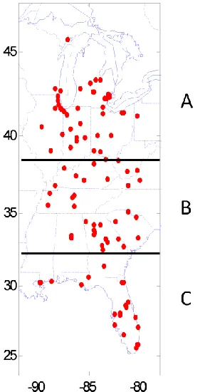
The models represent a single-source single-tier retail distribution network with aggregated
product information. The customer locations and the potential facility locations are the
three-digit ZIP codes for the continental U.S. with non-zero population (877 in total). The
geographical location of each three-digit ZIP code is taken to be the population centroid of
its constituent five-digit ZIP codes. The customer weights are proportional to population
densities. In generating the costs for the models we assume the supply chain mirrors
existing retail networks in the U.S., which typically contain between five and thirty
warehouses to serve most of the continental U.S. For example, Lowe‘s Companies [2006]
11 serve the continental U.S. The great circle distance in statute miles, magnified by a circuity
factor of 1.2, is used to determine the distance between facilities and customer locations
[Ballou et al. 2002].
The following notation is used. Let N 1, 2,,877 be the (arbitrarily) ordered set of all
customer locations (i.e., such that N 877). For each problem instance that is modeled
and solved, we define Nn N ( Nn n) to be the customer location set, with
60,100, 400, 600,877
n representing the instance sizes that are ultimately formulated and
solved in this research. Further, let M Nn be the set of m candidate facility locations (i.e.,
M m) for a particular problem. In all cases we use M Nn (such that m n); however,
in some subroutines we refer to instances with M Nn (such that m n). Also, a range of
scale exponents b 0, 0.35, 0.5 are tested for Equation (2.2).
We develop and assess solution methods through a series of empirical studies. The values
of b that were tested (0, –0.35, and –0.5) were chosen, respectively, to represent no
economies of scale, a typical manufacturing economy of scale, and the square root law for
inventory. To evaluate a wide range of problems and parameters, smaller problems ranging
from 60 – 600 customers were generated by sampling from the 877 customer problem set
using a random weighted permutation with the customer demand normalized to maintain a
total demand of 1.5 million units per year. The heuristic models were created and executed
in MATLAB 7.2, utilizing Matlog as a building block for the models [Kay 2006]. CPLEX
10.0 was used to solve the integer and mixed integer formulations. All tests were run on a
12 4.2 Metaheuristic Solution Approaches for Smaller Problems
To assess each heuristic we compare solution cost, solution time, and computational effort.
We allow each heuristic to run to completion—until there is no improvement in total cost or
until the program terminates due to the computer being out of memory (OoM). We
developed three measures of computational effort. These measures count the number of
computational evaluations needed to reach a solution. We consider these evaluation
measurements to be more important measures of efficiency than solution time as they better
predict the algorithm behavior as the complexity of the objective function increases. Each
measure counts each evaluation of the nonlinear facility cost, computationally the most
expensive cost to calculate in our problem formulation. As we discuss below, in an attempt
to reduce the number of evaluations, a simplified cost function is utilized in some of the
heuristic subroutines. These steps only include fixed facility costs and/or transportation
costs.
We, characterize the evaluation measurements into three categories that count the number of
objective function evaluations: construction evaluations, allocation evaluations, and location
evaluations. An allocation evaluation is defined as each instance in which a customer
allocation is attempted for each facility in the allocation subroutine. A construction
evaluation is the same computationally as an allocation evaluation, except that it occurs in
the ADD/construction subroutine. In some cases we report these two measures as a
combined measure: however, we track them separately to gain a deeper understanding of the
behavior of the heuristics. A location evaluation is each instance, within the location
subroutine, in which the algorithm evaluates the re-location of a facility to another location.
We first test a set of heuristics on smaller sized instances with n=60 and 100. This set was
reduced in the later empirical study to include those methods that offered the best
13 are summarized in Table 1. The first heuristic, AD-dALA, is an adaptation of the add/drop
heuristics described by Daskin [1995] for the UFLP combined with a discrete ALA
improvement procedure. In this approach the construction algorithm adds facilities
considering only fixed facility costs and transportation costs to obtain a set of starting
facility locations and set an upper bound on the number of facilities to locate. A greedy
DROP procedure is then used to remove facilities from the solution until the total cost is no
longer reduced.
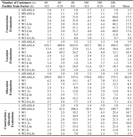
Table 1: Metaheuristics Analyzed on Smaller Instances
Heuristic
Facility Add/ Construction
Customer
Allocation Facility Location 1. AD-dALA Add with no scale costs,
followed by Drop
procedure with scale costs
All customers Fixed Neighborhood Search (FNS) using Delaunay triangulation
2. MS -dALA AD solution provides range in p values to test
Same as heuristic 1
Same as heuristic 1
3. W1 Greedy Add using all
unused locations
Same as heuristic 1
FNS checking all locations in the subgraph
4. W2 Same as heuristic 3 Same as
heuristic 1
Same as heuristic 1
5. W1-LAt Same as heuristic 3 Only customers on
convex hull of the current allocation
Same as heuristic 3, but only assess subgraphs with new facility allocations
6. W2- Lt Same as heuristic 3 Same as
heuristic 1
Same as heuristic 1, but only assess subgraphs with new facility allocations
7. W2-LAt Same as heuristic 3 Same as
heuristic 5
Same as heuristic 6
8. W1-S Generate subset using
simplified Whitaker ADD procedure from heuristic 3. Then use same procedure as heuristic 3
Same as heuristic 1
Same as heuristic 3
9. W2-S-LAt Same as heuristic 8 Same as
heuristic 5
Same as heuristic 6
Our DROP procedure is identical to that offered by Daskin, except in that our procedure
14 from the previous iteration? to determine the marginal facility unit cost. At the end of the
DROP procedure, if one or more facilities have no retailers assigned to them, these facilities
are removed to avoid a degenerate solution [Brimberg and Mladenovic 1999]. After the
DROP procedure is complete, a discrete ALA improvement procedure is used. This
procedure is an adaptation of the continuous location heuristic described by Bucci and Kay
[2006]. Our discrete version differs from their heuristic by constraining the possible facility
locations (m) to the set of customer locations, incorporating fixed facility location costs, and
using a Delaunay triangulation (DT) discrete neighborhood relocation search in place of the
continuous location search. Since the local neighborhood search may not yield the optimal
facility locations for the allocation, the location procedure is re-run until there is no
improvement in the solution.
Regarding the allocation procedure, the first allocation evaluation includes only
transportation and fixed facility costs to allocate the customers to the facilities since we have
not yet determined a facility size to calculate the marginal facility costs. Using this
allocation, the marginal facility cost is then added to obtain a total cost for the current
solution. In subsequent allocation cycles, the facility sizes from the previous allocation
cycle are used to establish the marginal facility costs for the next allocation cycle with no
updates to the facility costs within the allocation cycle. As in the location procedure, we
re-run the allocation cycle until there is no further improvement in the solution. The
location-allocation iterations continue until there is no improvement in total cost. To avoid a
degenerative condition [Brimberg and Mladenovic 1999] we check for unused facilities after
each allocation cycle and randomly relocate any unused facility prior to the next location
cycle.
The second model, MS-dALA, is an adaptation of the d-eosALA procedure [Bucci et al.
2007] that uses the result of the ADD/DROP initialization procedure described above to
determine a range for the number of facilities (p) to locate. Since this initialization may not
15 we evaluate solutions with the optimal number of facilities. Using the results from Bucci
and Kay [2006] and Houck et al. [1996], which provide guidance on the number of re-starts
for random start ALA procedures, we perform forty random starts at each value of p. The
discrete ALA procedure is identical to the procedure in the AD-dALA heuristic. At the end
of the improvement procedure unused facilities are dropped from the solution. We use this
MS-dALA procedure as a baseline for the other heuristics as it closely resembles the
multi-start ALA procedure commonly used in facility location problems [Brimberg et al. 2000].
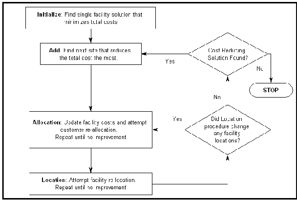
The third heuristic (W1) is a minor variant of the ADD algorithm described by Whitaker
[1985]. Whitaker‘s heuristic is a modification of a greedy ADD procedure that includes an
iterated location-allocation improvement procedure between each construction step.
Adding a facility in each cycle is based first on the transportation and fixed cost; only
afterwards are marginal facility costs added to establish a total cost for the solution. Like
the d-eosALA heuristic, the W1 heuristic uses the facility sizes from the previous allocation
cycle to determine the nonlinear facility costs for the current solution. The allocation
procedure evaluates all retail customers in each cycle. The location procedure considers all
customer locations in the subgraph as possible relocation sites for each facility. To reduce
the possibility that the model will terminate prematurely, this process of
ADD-allocate-locate continues until there are three solutions that are not better than the current best
16 Figure 1: Solution Procedure for W1 Heuristic
Heuristics four to nine are modifications of the W1 procedure with changes in the
ADD/construction, location, and/or allocation procedures in an attempt to reduce the
computational evaluations without a significant degradation in the solution. The fourth
heuristic (W2) differs from the W1 heuristic in utilizing the same Delaunay triangulation
neighborhood search used in the AD-dALA heuristic. An example of the re-location set for
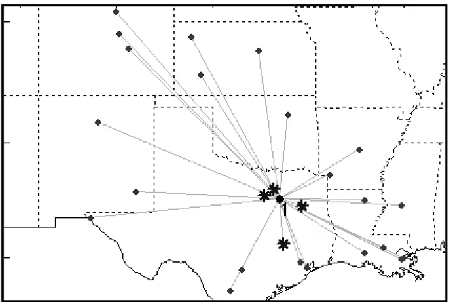
one subgraph is shown in Figure 2. The locations labeled with either an asterisk or a dot (27
in total) are assessed in the W1 re-location search, while only the locations labeled with an
17 Figure 2: Example of a re-location set for the W1 and W2 Heuristics
The fifth heuristic (W1-LAt) differs from the W1 heuristic in both the location and
allocation search. It was observed in early testing that the allocations for some facilities did
not change in each location cycle, therefore, performing the re-location search for these
facilities was unnecessary. To address this situation this heuristic incorporates a Tabu
Search (TS) concept, short term memory, by storing the allocation from the previous cycle
and only performs a re-location search in subgraphs in which the allocation has changed. In
the allocation procedure only customers along the convex hull of the allocation are
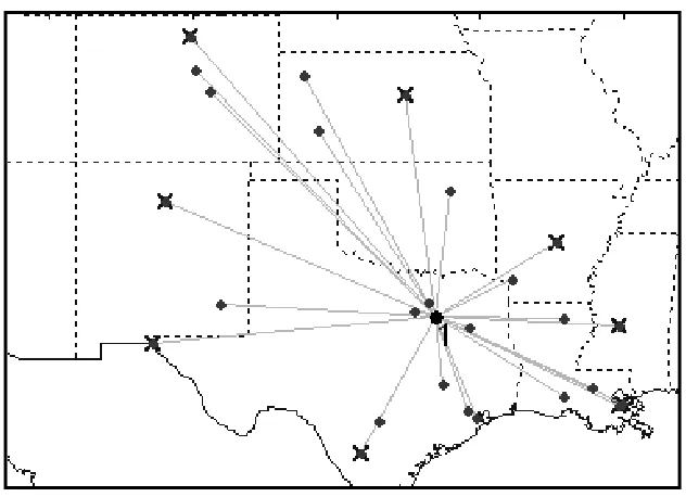
considered. An example of the re-allocation set for one subgraph is shown in Figure 3. The
locations labeled with either a ―x‖ or a dot (27 in total) are assessed in the W1 re-allocation
search, while only the locations labeled with an asterisk (9 in total) are assessed in the
W1-LAt convex hull re-allocation search. The W2-Lt heuristic adds the short term memory
improvement to the W2 heuristic. The W2-LAt heuristic extends the W2-Lt heuristic by
18 Figure 3: Example of a re-allocation set for the W1 and W1-LAt Heuristics
Heuristic 8 (W1-S) varies from the W1 heuristic only in the construction procedure. Rather
than searching every unused facility location in the construction procedure, this heuristic
only searches a subset of the unused facility locations, M Nn (such that m n m, 100).
We use the W1 heuristic with a simplified objective function containing only transportation
and fixed facility costs in an attempt to intelligently create the subset locations. The subset
size ms is defined by the following. The simplified W1 heuristic runs until there is no improvement in total cost and ms 0.25n, however, the size of ms is capped at ms 100. We set ms 100 based on the clustering analysis research from Ballou [1994] who studied a
similar customer location dataset. We set m 0.25n based on limited results showing this
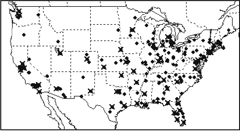
percentage did not exhibit a noticeable increase (0.001%) in the objective function. Figure 4
provides an example of the construction subset for a problem with n = 200 and ms = 50. The locations with either a ―x‖ or a dot is the complete possible facility set, while the locations with a ―x‖ are in the subset. The final heuristic, W2-S-LAt, applies the subset in the
19 To improve the evaluation of the heuristics CPLEX 10.0 was used where possible to find
optimal solutions. Early tests showed CPLEX could not find an optimal solution for
problems with n ≥ 100 using a three segment piecewise approximation; however, with b =
0.0 and the problem formulated as an integer program (IP) CPLEX quickly finds an optimal
solution. Therefore, for problems with n ≥100 CPLEX was used as a comparison for the
heuristics for all problems with b = 0.0.
20 4.3. Performance of Metaheuristics on Smaller Problems
Given that the dataset is new, we use the MS-dALA procedure as an indicator of the
difficulty of the problem as multi-start procedures are a common baseline comparison for
facility location problems [Houck et al. 1996, Brimberg et al. 2000]. We define a ―good‖
solution to be less than 1% from the best solution found over all algorithms used. For
n=100, b= 0.35 the MS-dALA procedure did not find any solutions within 2% of the best
solution and on average was 11% from the best solution, thus allowing us to conclude the
problems are significantly challenging to solve within 1% of the best known value.
For each test instance, we compute total cost, solution time, and the three measures of
computational effort. The total cost was analyzed using a ―percent above best‖ (%AB)
measurement that has been used in facility location research [Brimberg et al. 2000].
Solution time and several evaluation measurements were analyzed using a ―multiple from
best‖ (xFB) measurement which is calculated by taking the heuristic value and dividing it by
the best value found among all of the heuristics. This offers an intuitive relative comparison
of solution time and number of evaluations required for the algorithms. A value of 1.0
means the heuristic achieved the best value.
Initial tests were conducted with n 60,100 using a random weighted permutation of the
877 customer dataset where weights were proportional to population densities. Ten
problems were generated at each value of n and with b 0, 0.35, 0.5 to obtain ten data
points at each (n,b) pair. For all problems with b = 0.0, CPLEX found an optimal solution.
For n = 60 and b = 0.5, 0.35 CPLEX was able to find optimal solutions; however, the
solution time was quite long (> 1 hr). For n = 100 and b = 0.35, CPLEX could not find an
optimal solution; however, the best CPLEX solution found and the best heuristic solution
are within 0.2% of each other. Our analysis compares the average of the ten tests. The total
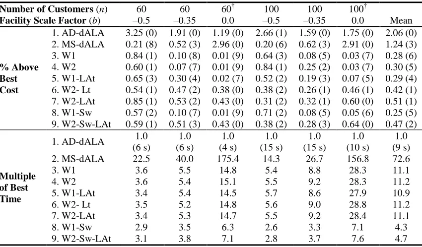
21 Table 2: Comparison of Average Total Cost and Average Solution Time
Number of Customers (n) 60 60 60† 100 100 100†
Facility Scale Factor (b) –0.5 –0.35 0.0 –0.5 –0.35 0.0 Mean
% Above Best Cost
1. AD-dALA 3.25 (0) 1.91 (0) 1.19 (0) 2.66 (1) 1.59 (0) 1.75 (0) 2.06 (0) 2. MS-dALA 0.21 (8) 0.52 (3) 2.96 (0) 0.20 (6) 0.62 (3) 2.91 (0) 1.24 (3) 3. W1 0.84 (1) 0.10 (8) 0.01 (9) 0.64 (3) 0.08 (5) 0.03 (7) 0.28 (6) 4. W2 0.60 (1) 0.07 (7) 0.01 (9) 0.84 (1) 0.25 (2) 0.03 (7) 0.30 (5) 5. W1-LAt 0.65 (3) 0.30 (4) 0.02 (7) 0.52 (2) 0.19 (3) 0.07 (5) 0.29 (4) 6. W2- Lt 0.54 (1) 0.47 (2) 0.38 (0) 0.38 (2) 0.26 (1) 0.46 (1) 0.42 (1) 7. W2-LAt 0.85 (1) 0.53 (2) 0.43 (0) 0.31 (2) 0.32 (1) 0.60 (0) 0.51 (1) 8. W1-Sw 0.57 (2) 0.10 (7) 0.01 (9) 0.71 (2) 0.08 (5) 0.05 (6) 0.25 (5) 9. W2-Sw-LAt 0.59 (1) 0.51 (3) 0.43 (0) 0.38 (2) 0.28 (3) 0.64 (0) 0.47 (2)
Multiple of Best Time
1. AD-dALA 1.0
(6 s) 1.0 (6 s) 1.0 (4 s) 1.0 (15 s) 1.0 (15 s) 1.0 (10 s) 1.0 (9 s)
2. MS-dALA 22.5 40.0 175.4 14.3 26.7 156.8 72.6
3. W1 3.6 5.5 14.8 5.4 8.8 28.3 11.1
4. W2 3.6 5.4 15.1 5.5 9.2 28.3 11.2
5. W1-LAt 3.4 5.4 14.5 5.7 8.6 27.9 10.9
6. W2- Lt 3.5 5.2 14.8 5.6 9.0 28.8 11.2
7. W2-LAt 3.4 5.3 14.7 5.5 9.2 28.4 11.1
8. W1-Sw 2.9 3.5 6.3 2.6 3.3 7.1 4.3
9. W2-Sw-LAt 3.1 3.8 7.1 2.8 3.7 7.6 4.7
†Best cost obtained via CPLEX
In Table 2, the values in parentheses for the cost measurement are the number of times the
best solution (within 0.05%) was found out of the ten runs. In the solution time section, the
second row of data for the AD-dALA heuristic is the average solution time in seconds. To
assess the statistical difference in cost between the heuristics we compare the distribution of
the %AB cost measurement for the thirty total tests with n = 100 and b 0, 0.35, 0.5
using a non-parametric Wilcoxon rank-sum test [Siegel 1994]. These results, not shown
here to conserve space, are consistent with the general results observable in Table 2. Table
3 reports the evaluation measurements for each algorithm. In Table 3 we also show the
allocation and construction evaluations as a combined measurement to provide a more
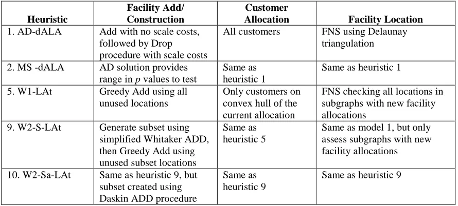
22 Table 3: Comparison of the Average Number of Evaluations using xFB Measurement
The following general observations from the analysis of these smaller instances will be used
in the analysis of larger problems.
OBSERVATION 1: The AD-dALA procedure provides solutions within 10% of the best
found solution with the fastest solution time and a relatively low number of evaluations. Number of Customers (n) 60 60 60 100 100 100
Facility Scale Factor (b) –0.5 –0.35 0.0 –0.5 –0.35 0.0 Mean
Co ns truct io n E v a lua tio ns
1. AD-dALA 1.6 1.1 1.0 1.7 1.1 1.0 1.3
2. MS-dALA 1.6 1.1 1.0 1.7 1.1 1.0 1.3
3. W1 2.6 3.0 31.0 4.0 4.4 60.0 17.5
4. W2 2.6 3.0 31.0 4.1 4.6 60.0 17.5
5. W1-LAt 2.5 3.0 31.0 4.2 4.4 60.1 17.5
6. W2- Lt 2.6 2.9 31.1 4.1 4.5 61.3 17.8
7. W2-LAt 2.5 3.0 31.2 4.0 4.6 60.0 17.6
8. W1-S 1.1 1.1 9.4 1.0 1.1 11.0 4.1
9. W2-S-LAt 1.0 1.1 8.8 1.0 1.1 9.7 3.8
L o ca tio n E v a lua tio ns
1. AD-dALA 1.7 1.9 3.2 1.2 1.3 1.8 1.9
2. MS-dALA 476.7 609.6 1015.0 243.2 381.2 494.5 536.7
3. W1 13.4 16.5 23.9 11.1 15.6 18.6 16.5
4. W2 6.8 10.3 24.2 3.4 6.0 12.1 10.5
5. W1-LAt 2.9 3.2 2.8 2.9 3.3 2.0 2.8
6. W2- Lt 1.7 2.0 1.5 1.4 1.7 1.6 1.6
7. W2-LAt 1.4 1.9 1.0 1.4 1.7 1.3 1.5
8. W1-S 13.5 16.3 24.0 11.6 15.7 18.3 16.6
9. W2-S-LAt 1.5 2.0 1.0 1.4 1.6 1.2 1.5
Allo ca tio n E v a lua tio ns
1. AD-dALA 1.0 1.0 1.0 1.2 1.0 1.0 1.0
2. MS-dALA 258.9 282.3 337.6 178.8 250.1 275.2 263.8
3. W1 6.2 8.6 14.1 4.7 7.8 13.1 9.1
4. W2 5.7 7.9 13.7 3.9 7.3 12.3 8.5
5. W1-LAt 2.4 4.1 8.0 1.6 2.9 7.1 4.4
6. W2- Lt 5.5 7.1 13.8 3.8 7.0 12.6 8.3
7. W2-LAt 2.5 3.9 7.7 1.3 3.2 7.2 4.3
8. W1-S 6.9 8.6 14.2 5.1 7.8 12.8 9.2
9. W2-S-LAt 2.7 3.9 7.7 1.5 3.1 7.1 4.3
Co ns truct io n + Allo ca tio n E v a lua tio ns
1. AD-dALA 2.7 1.0 1.0 1.4 1.0 1.0 1.4
2. MS-dALA 3.9 42.5 206.4 29.5 36.3 189.7 84.7
3. W1 7.7 3.5 19.2 3.7 4.5 25.4 10.7
4. W2 7.1 3.3 18.9 3.7 4.6 24.9 10.4
5. W1-LAt 3.1 2.8 15.5 3.4 3.8 21.3 8.3
6. W2- Lt 4.3 3.2 19.1 3.7 4.5 25.5 10.0
7. W2-LAt 2.1 2.7 15.4 3.2 4.1 21.4 8.1
8. W1-S 1.5 2.0 11.8 1.6 1.9 11.8 5.1
23 This is primarily due to the computationally simple ADD/DROP method used in the
construction procedure.
OBSERVATION 2: The MS-dALA procedure provides better quality solutions than the
AD-dALA, but this improvement comes with a large increase in both location and allocation
evaluations due to the large number of multi-starts needed to obtain a good solution.
Additionally, the solutions for the MS-dALA procedure degrade as b 0 and the number
of facilities in the solution increases. This result is consistent with studies of multi-start
ALA procedures [Brimberg et al. 2000, Hansen et al. 1998].
OBSERVATION 3: Using the tabu search techniques we see a statistically significant
increase in total cost, however, the difference is small in practical terms (on average all
solutions are within 0.25% of each other using the %AB measure). This minor degradation
in solution quality brings a significant reduction in location and allocation evaluations. In
contrast to the MS-dALA procedure heuristics three to seven show improvement in the total
cost as the number of facilities in the solution increases due to the iterative construction and
improvement nature of the heuristics [Whitaker 1985].
OBSERVATION 4: By using a subset of facilities in the construction procedure we
achieve a significant reduction in total allocation evaluations with only a minor degradation
in the objective function (as compared to heuristics three and four). This result is consistent
with variable neighborhood search studies, which show the use of multiple neighborhoods
with a local improvement procedure is an effective combinatorial approach [Hansen and
Mladenovic 1997].
OBSERVATION 5: The measurement of computational effort in each procedure
(construction, location, and allocation) has added significantly to our understanding of the
behavior of the heuristics. By using these measures we are better able to predict the
24 4.4 Metaheuristic Solution Approaches for Larger Problems
Based on the observations from the study of smaller instances a subset of the heuristics are
tested on larger instances with n 200, 400, 600,877 and b 0, 0.35, 0.5 . The
instances are generated using the same parameters and methods as in the n 60,100
study. Due to longer solution times only one test for each (n,b) pair is performed. Table 4
summarizes the heuristics analyzed. To avoid confusion, we use the same numbering of
solution methods as in Table 1. Heuristic ten is a modification of heuristic nine that
employs a different approach to create the subset of facility locations for use in the
construction procedure. Using the same criteria used in the construction subset creation in
heuristic nine, heuristic ten uses the Daskin ADD procedure used in Heuristic one to
generate the construction subset facility locations.
Table 4: Heuristics Analyzed on Larger Instances
Heuristic
Facility Add/ Construction
Customer
Allocation Facility Location 1. AD-dALA Add with no scale costs,
followed by Drop
procedure with scale costs
All customers FNS using Delaunay triangulation
2. MS -dALA AD solution provides range in p values to test
Same as heuristic 1
Same as heuristic 1
5. W1-LAt Greedy Add using all unused locations
Only customers on convex hull of the current allocation
FNS checking all locations in subgraphs with new facility allocations
9. W2-S-LAt Generate subset using simplified Whitaker ADD, then Greedy Add using unused subset locations
Same as heuristic 5
Same as model 1, but only assess subgraphs with new facility allocations
10. W2-Sa-LAt Same as heuristic 9, but subset created using Daskin ADD procedure
Same as heuristic 9
Same as heuristic 9
4.5 Performance of Metaheuristics on Larger Problems
CPLEX continued to provide optimal solutions for all IP formulations of the problem (b =
25 Total cost and solution time for the n 200, 400, 600,877 problems are reported in Table
5. Within the ―Multiple of Best Time‖ section of the table, the second row of data for the
AD-dALA heuristic is the average solution time in seconds. In some problems the heuristics
were unable to reach a final solution due to an ―out of memory‖ error, which we depict with ―--‖ in the tables. Heuristics five and nine cannot solve the largest problems (n = 877).
Heuristic five causes an out of memory error in the construction procedure as it attempts to
add the second facility to one of the 877 facility locations. Heuristic nine causes an out of
memory error in the creation of the construction. The measurements of computational effort
are shown in Table 6.
Table 5: Comparison of Average Total Cost and Average Solution Time
Number of Customers (n) 400 400 400† 600 600 600† 877 877 877† Facility Scale Factor (b) -0.5 -0.35 0.0 -0.5 -0.35 0.0 -0.5 -0.35 0.0
% Above Best Cost
1. AD-dALA 0.22 2.80 5.24 1.22 1.60 1.76 4.23 0.00 1.79
2. MS -dALA 0.00 0.04 3.00 0.00 0.55 2.06 0.00 1.33 2.18
5. W1-LAt 1.13 0.00 0.20 3.33 0.00 -- -- -- --
9. W2-Sw-LAt 0.61 0.41 0.41 0.58 0.12 2.07 -- -- --
10. W2-Sa-LAt 0.65 0.12 0.00 0.58 0.00 0.12 4.05 0.00 0.09
Multiple of Best Time
1. AD-dALA 1.0
254s. 1.0 231s. 1.0 110s. 1.0 566s. 1.0 495s. 1.0 250s. 1.0 1366s. 1.0 1270s. 1.0 627s.
2. MS -dALA 6.4 14.6 93.0 15.1 73.8 7.33 9.4 54.8
5. W1-LAt 18.6 32.1 162.8 24.4 50.8 -- -- -- --
9. W2-Sw-LAt 11.7 16.5 55.5 7.3 26.3 65.2 -- -- --
10. W2-Sa-LAt 5.3 9.4 41.9 8.6 10.6 45.0 5.0 9.9 40.7
†
Best cost obtained via CPLEX
Analyzing the results of the larger problems the following general observations can be
made, some of which parallel our findings in the smaller problem study.
OBSERVATION 1: The AD-dALA procedure provides solutions within 6% of the best
found solution with a relatively low number of evaluations and fast solution time. Solution
quality for the AD-dALA procedure improves as b→0.0. This algorithm may be a viable
alternative if a larger margin of error in the solution is acceptable and a low number of
26 OBSERVATION 2: The MS-dALA procedure provides better solutions on average than the
AD-dALA, but this improvement comes with a large increase in solution time and the
number of evaluations required due to the large number of multi-starts needed to obtain a
good solution. The solution quality of this procedure, as expected, deteriorates as the
number of facilities in the final solution increases.
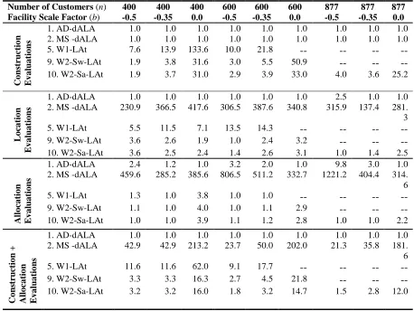
Table 6: Comparison of the Average Number of Evaluations using xFB Measurement
Number of Customers (n) 400 400 400 600 600 600 877 877 877 Facility Scale Factor (b) -0.5 -0.35 0.0 -0.5 -0.35 0.0 -0.5 -0.35 0.0
Co ns truct io n E v a lua tio ns
1. AD-dALA 1.0 1.0 1.0 1.0 1.0 1.0 1.0 1.0 1.0
2. MS -dALA 1.0 1.0 1.0 1.0 1.0 1.0 1.0 1.0 1.0
5. W1-LAt 7.6 13.9 133.6 10.0 21.8 -- -- -- --
9. W2-Sw-LAt 1.9 3.8 31.6 3.0 5.5 50.9 -- -- --
10. W2-Sa-LAt 1.9 3.7 31.0 2.9 3.9 33.0 4.0 3.6 25.2
L o ca tio n E v a lua tio ns
1. AD-dALA 1.0 1.0 1.0 1.0 1.0 1.0 2.5 1.0 1.0
2. MS -dALA 230.9 366.5 417.6 306.5 387.6 340.8 315.9 137.4 281. 3
5. W1-LAt 5.5 11.5 7.1 13.5 14.3 -- -- -- --
9. W2-Sw-LAt 3.6 2.6 1.9 1.0 2.4 3.2 -- -- --
10. W2-Sa-LAt 3.6 2.5 2.4 1.4 2.6 3.1 1.0 1.4 2.5
Allo ca tio n E v a lua tio ns
1. AD-dALA 2.4 1.2 1.0 3.2 2.0 1.0 9.8 3.0 1.0
2. MS -dALA 459.6 285.2 385.6 806.5 511.2 332.7 1221.2 404.4 314. 6
5. W1-LAt 1.3 1.0 3.8 1.0 1.0 -- -- -- --
9. W2-Sw-LAt 1.1 1.0 4.0 1.0 1.1 2.9 -- -- --
10. W2-Sa-LAt 1.0 1.0 3.9 1.1 1.2 2.8 1.0 1.0 2.2
Co ns truct io n + Allo ca tio n E v a lua tio ns
1. AD-dALA 1.0 1.0 1.0 1.0 1.0 1.0 1.0 1.0 1.0
2. MS -dALA 42.9 42.9 213.2 23.7 50.0 202.0 21.3 35.8 181.
6
5. W1-LAt 11.6 11.6 62.0 9.1 17.7 -- -- -- --
9. W2-Sw-LAt 3.3 3.3 16.3 2.7 4.5 21.8 -- -- --
10. W2-Sa-LAt 3.2 3.2 16.0 1.8 3.2 14.7 1.5 2.8 12.0
OBSERVATION 3: The use of a subset in the construction procedure and the method to
create this subset are critical factors to be able to solve large problems. Moreover, the use of
a subset has a negligible impact on solution quality. This result is consistent with Ballou‘s
27 OBSERVATION 4: Combining the subset in the construction procedure and tabu search
techniques in the location and allocation procedures clearly provides the best overall
solution cost for the range of problems tested and requires only a moderate number of
evaluations. Solution quality for this procedure (heuristic 10) improved as b→0.0 due to the
iterative construction and improvement nature of the heuristic. For problems with n ≥ 400
where optimal values were found (b = 0.0), this algorithm was within 0.12% of the optimal
value on average. Although this procedure requires a longer solution time relative to the
AD-dALA heuristic, the number of evaluations to generate a solution, however, is similar
for most problems suggesting that this heuristic should achieve similar solution times as the
cost function becomes more complex.
5. Conclusions and Directions for Future Work
In this paper several integrative metaheuristics solution methods for large scale facility
location problems that include non-linear costs that can represent risk pooling and/or
production economies of scale are presented. The solution approaches are extensions of
well studied methods used for the multi-source Weber, P-median, and uncapacitated fixed
charge facility location problems. Using an empirical study a large test bed of problems was
developed, that included some optimal solutions obtained using CPLEX, for comparing the
solution approaches over a range of problem sizes. The metaheuristics combined ADD,
DROP, ALA, variable neighborhood search, multi-start, and tabu search techniques. We
showed that measuring the number of computational evaluations provided insight into the
behavior of the heuristics that is not apparent when only using solution time and total cost.
Specifically, these measures showed that the use of tabu search techniques in the location
and allocation subroutines, and the creation of a subset of possible new facility locations in
the add/construction subroutine both significantly reduced the evaluations required with
minimal impact on solution quality. The advantage of each of these techniques was
correlated with the number of facilities in the final solution.
28 There are several avenues for future research. The concepts of Tabu search can be extended
in the location and allocation procedures in an attempt to further reduce the computational
evaluations required. Adding VNS and/or TS to supplement and/or replace the multi-start
procedure may make the discrete ALA metaheuristic more viable as these techniques have
been successfully implemented in p-Median problems [Hansen and Mladenovic 1997,
Brimberg et al. 2000]. Finally, as the metaheuristics are flexible in the type of cost function
that can be solved, the models can be extended to include both strategic and tactical level
decisions as well as capture other relevant cost parameters not included in typical facility
location models; for example uncertainty in supply and demand, and demand correlation.
6. Acknowledgments
This research is supported, in part, by the National Science Foundation under Grant
CMS-0229720 (NSF/USDOT).
7. References
1. Ballou, R.H., Rahardja, H., Sakai, N., 2002, Selected country circuity factors for road travel distance estimation, Transportation Research Part A, 36, 843-848.
2. Ballou, R.H., 1994, Measuring Transport Costing Error in Customer Aggregation for Facility Location, Transportation Journal, 33, 49-59.
3. Bischoff, M., Dachert, K., 2009, Allocation search methods for a generalized class of location allocation problems, European Journal of Operational Research, 192, 793-807.
4. Brimberg, J.,Hansen, P., Mladenovic, N.,Taillard, E.D. ,2000, Improvements and Comparison of Heuristics for Solving the Uncapacitated Multisource Weber Problem, Operations Research, 48, 444–460.
29 6. Bucci, M.J., Kay, M.G., 2006, A Modified ALA Procedure for Logistic Network
Designs with Scale Economies, Industrial Engineering Research Conference, IERC 2006, Orlando Florida.
7. Bucci, M.J., Kay, M.G., Waring, D.P., 2007, A Comparison of Meta-Heuristics for Large Scale Facility Location Problems with Economies of Scale, Industrial Engineering Research Conference, IERC 2007, Nashville, Tennessee.
8. Cooper, L., 1963, Location-allocation problems, Operations Research, 11, 331–343.
9. Croxton, K.L., Zinn,W., 2005, Inventory Considerations in Network Design, Journal of Business Logistics, 26, 149-168.
10. Daganzo, C.F., 2005, Logistics systems analysis, Springer, New York, NY.
11. Daskin, M.S., Coullard, C.R., Shex, Z.M., 2002, An Inventory-Location Model: Formulation, Solution Algorithm and Computational Results, Annals of Operations Research, 110, 83-106.
12. Daskin, M.S.,1995, Network and discrete location: models, algorithms, and applications, John Wiley and Sons, New York.
13. Gendreau, M., Potvin, J.Y., 2005, Metaheuristics in combinatorial optimization, Annals of Operations Research, 140, 189-213.
14. Glover, F., Laguna, M., 1997, Tabu Search, Kluwer Academic Publishers, Boston, MA.
15. Hansen, P., Mladenovic, N., Taillard, E., 1998, Heuristic solution of the multisource Weber problem as a p-median problem, Operations Research Letters, 22, 55–62.
16. Hansen, P., Mladenovic, N., 1997, Variable Neighborhood Search for the P-median, Location Science, 5, 207–226.
17. Houck, C.R., Joines, J.A., Kay, M.G., 1996, Comparison of genetic algorithms, random restart and two-opt switching for solving large location-allocation problems, Computers and Operations Research, 23, 587-796.
30 19. Kay, M.G., 2006, Matlog: Logistics Engineering Toolbox, North Carolina State
University (http://www.ie.ncsu.edu/kay/matlog).
20. Lowe‘s Companies, Inc., 2006 Annual Report, http://www.shareholder.com/lowes/annual.cfm
21. Maister, D.H., 1976, Centralization of Inventories and the ‗Square Root Law,‘ International Journal of Physical Distribution, 6, 124-134.
22. Melachovsky, J., Prins, C., Calvo, R.W., 2005, A Metaheuristic to Solve a Location-Routing Problem with Non-Linear Costs, 11, 375–391.
23. Mirchandani, P.B., Francis, R.L., 1990, Discrete Location Theory, Wiley, New York.
24. Perl, J., Daskin, M.S., 1985, A Warehouse Location-Routing Problem, Transportation Research Part B, 19, 381–396.
25. Resende, M.G.C., Werneck, R.F., 2006, A hybrid multistart heuristic for the
uncapacitated facility location problem, European Journal of Operational Research, 174, 54–68.
26. Rumelt, R.P., 2001, Note on Strategic Cost Dynamics, POL 2001-1.2, Anderson School at UCLA, pp. 2–3.
27. Siegel, A.F., 1994, Practical Business Statistics, Irwin, Burr Ridge, Ill.
28. Walgreen Company, 2006 Annual Report, http://www.shareholder.com/lowes/annual.cfm
29. Whitaker, R.A. 1985 Some Add-Drop and Drop-Add Interchange Heuristics for Non-Linear Warehouse Location, The Journal of the Operational Research Society, 36, 61–70.
31 CHAPTER 3: Modeling Inventory Pooling Effects in Facility Location
Michael J. Bucci*, Michael G. Kay*, Donald P. Warsing†, Reha Uzsoy*, James R. Wilson*
*Fitts Department of Industrial and Systems Engineering, North Carolina State University, Raleigh, NC 27695, USA †
Department of Business Management, North Carolina State University, Raleigh, NC 27695, USA
32
Modeling Inventory Pooling Effects in Facility Location
Michael J. Bucci*, Michael G. Kay*, Donald P. Warsing†, Reha Uzsoy*, James R. Wilson*
*Fitts Department of Industrial and Systems Engineering, North Carolina State University, Raleigh, NC 27695, USA †
Department of Business Management, North Carolina State University, Raleigh, NC 27695, USA
Abstract
We investigate the ―Square Root Law‖ (SRL) and a more general concave cost function for computing inventory levels that account for pooling effects in facility location models. We compare inventory levels, total cost, solution time, and solution structure (facility locations and allocations) to solutions that use the explicit safety stock inventory calculation. For models with no correlation in demand across customer locations, we show that SRL poorly estimates the inventory required in many situations and the more general cost function always outperforms the SRL. Both approaches, however, result in underlying solution
structures that are close to the solution using the explicit calculation. We then extend our analysis to models that include inter-customer correlation in demand, demonstrating the degradation of both approximation approaches as inter-customer correlation increases, and suggesting that either the explicit computation of pooled inventory levels, or better methods of approximating them, are required to generate good solutions.
Keywords
Facility location, inventory pooling, safety stock, demand correlation
1. Introduction
We investigate large-scale facility location models that account for the risk pooling effects
associated with centralizing safety stocks. The models represent a single-source, single-tier
distribution network that may also exhibit correlation across customer demands. The
objective of the model is to locate an unknown number of distribution centers to minimize
the sum of transportation and safety inventory costs. Unlike traditional location models
[e.g., Daskin 1995], distribution networks have increasingly come to rely on contracts of
relatively short duration in which warehouse space is rented from third parties [Armstrong
and Associates 2009]. Thus, the customary fixed costs due to facility construction and
infrastructure are not incurred or are significantly reduced, although the firm may incur