Detecting marker-QTL linkage and estimating QTL gene effect and map location using a saturated genetic map.

(1)

Copyright 0 1993 by the Genetics Society of America

Detecting Marker-QTL Linkage and Estimating QTL Gene Effect and Map

Location Using a Saturated Genetic Map

A. Darvasi,* A. Weinreb,* V. Minke,*

J. I. Wellert and M. Soller*

*Department of Genetics, The Alexander Silberman Lqe Sciences Institute, The Hebrew University of Jerusalem, 91904 Jerusalem, Israel, and ?Animal Science Institute, Agricultural Research Organization, Volcani Center, 50250 Bet Dagan, Israel

Manuscript received September 25, 1992

Accepted for publication March 5, 1993

ABSTRACT

A simulation study was carried out on a backcross population in order to determine the effect of marker spacing, gene effect and population size on the power of marker-quantitative trait loci (QTL) linkage experiments and on the standard error of maximum likelihood estimates (MLE) of QTL gene effect and map location. Power of detecting a QTL was virtually the same for a marker spacing of 10 cM as for an infinite number of markers and was only slightly decreased for marker spacing of 20 or even 50 cM. T h e advantage of using interval mapping as compared to single-marker analysis was slight. “Resolving power” of a marker-QTL linkage experiment was defined as the 95% confidence interval for the QTL map location that would be obtained when scoring an infinite number of markers. It was found that reducing marker spacing below the resolving power did not add appreciably to narrowing the confidence interval. Thus, the 95% confidence interval with infinite markers sets the useful marker spacing for estimating QTL map location for a given population size and estimated gene effect.

S

AX (1923) was the first tQ show that quantitative trait loci (QTL) could be associated with marker loci in crosses between inbred lines. For many years paucity of suitable markers virtually limited these studies to Drosophila (e.g., SPICKETT and THODAY

1966). However, the advent of biochemical markers and more recently of DNA-level markers has seen the extension of such studies to other species (EDWARDS, STUBER and WENDEL 1987; KAHLER and WEHRHAHN 1986; NIENHUIS et al. 1987; OSBORN, ALEXANDER and FOBES 1987; PATERSON et al. 1988; WELLER 1987; WELLER, SOLLER and BRODY 1988).

Detecting marker-QTL linkage can be carried out through t-tests based on single markers (SOLLER, BRODY and GENIZI 1976) or by means of likelihood ratio tests (LRT) that involve the use of a pair of markers bracketing a Q T L , a procedure termed “interval mapping” (JENSEN 1989; KNAPP, BRIDGES and BIRKES 1990; LANDER and BOTSTEIN 1989; VAN OOI- JEN 1992). Estimating QTL map location, however,

will generally require application of methods for maximum likelihood estimation (MLE) (JENSEN 1989; KNAPP, BRIDGES and BIRKES 1990; LANDER and BOT- STEIN 1989; SIMPSON 1989; VAN OOIJEN 1992; WELLER 1987), although simpler approaches are possible (HALEY and KNOTT 1992; THODAY 196 1 ; WELLER 1987).

It should be noted that detecting marker-QTL linkage by LRT and estimating QTL map location by MLE are different procedures and should be treated as such. Although both can be carried out within the

Genetics 134: 943-951 (July, 1993)

same analysis, experimental parameters such as population size, Q T L effect and marker spacing may influence the two procedures differently.

Here, a comprehensive theoretical study is carried out in order to determine the effect of marker spacing on the power of marker-QTL linkage experiments and on the standard error of maximum likelihood estimates of Q T L gene effect and map location. T h e power of detecting marker-QTL linkage is investigated using interval mapping and LRT as a function of marker spacing and Q T L location relative to the closest flanking marker, as compared to the power of a multiple single-marker analysis using a simple t-test in the same genetic architecture. T h e standard errors (SE) of the maximum likelihood estimates (MLE) of the mean and variance, and confidence intervals for the estimated map location of the QTL are also obtained as a function of marker spacing. T h e power of marker-QTL linkage determination and the confidence interval for the QTL estimated map location, are then derived for the case where an infinite number of markers are scored. T h e study is carried out in a simulated backcross population. This experimental design was chosen because of its analytical simplicity and widespread use in practice. It is believed that the general principles derived from the simulation study will be applicable to other experimental designs as well.

THEORY

(2)

1

2

3

4

5

6

7

8

9

c

I

t

I I

I

t

I I

I

,

t

,

I I I

t ,

I I

, t ,

I I

I ' I l I' l I I l

) l I I I t ~ I I I ~ ~

I I I I I t I I I I I I

I I I I I i

0 20 40 60 80 100

cM

FIGURE 1.-Marker (bar) and QTL (inverted arrow) locations according to marker spacing: 50 cM (lines 1, 2, 3). 20 cM (lines 4,

5 , 6 ) and 10 cM (lines 7 , 8, 9), and location of Q T L relative to the markers: at the marker (lines 1 , 4 , 7 ) , '/4 of distance between markers (lines 2, 5, 8), and midway between the markers (lines 3, 6 , 9).

-The backcross population originates from a cross between two inbred lines that are homozygous at all differentiating marker loci and QTL.

-One Q T L is present in a chromosome of length 100 cM.

-The trait value has a normal distribution with means

p 1 and PZ for the two Q T L genotypes present in the backcross population and equal variance, a2, for both genotypes.

-Starting at 0, there is a marker every c cM along the chromosome and, marker locations are known on the basis of prior information.

-Crossing over interference is not present.

-The simulation population was generated for all combinations of p1 = 0; p z = 0.25, 0.5; cr2 = 1; N = 500, 1000; c = 0, 10, 20, 50 (c = 0 represents the model with an infinite number of markers) and the QTL was always located at the central interval with

k

= 0, l/4, '/2, where,

k

is the relative position of the

Q T L between its two flanking markers (Figure 1).

In addition, for the representative case of c = 20 cM

Darvasi al.

and the QTL located at the mid-point of the two central markers (12 = Y 2 ) , additional simulations were also carried out for p2 = 0.25, 0.5, 0.75, 1 .O and 1.5 with N = 100; and for N = 100, 200 and 2000 with

-For the simulations, 1000 replicates were generated pr, = 0.25.

for each parameter combination.

T h e backcross population was generated as follows. (i) For each individual one chromosome was generated according to the given assumptions. (ii) T h e genotypes of the markers and the Q T L were sampled from a binomial distribution according to the proportions of recombination between markers and QTL. (iii) Ac- cording to the Q T L genotype sampled, the trait value was sampled from a normal distribution with the corresponding mean.

Markers spaced at intervals

Single marker analysis: At each marker a t-test was carried out to determine significance of the difference between the averages of the homozygous and the heterozygous individuals for that marker. If a significant difference was detected at any marker it was considered as a Q T L detected in that simulation. Each individual t-test was carried out on an individual marker. Therefore, a per-marker type I error was required, defined in a way to control the per-chromosome type 1 error (ie., the probability that in a given chromosome a Q T L will be detected when none is present). Controlling the overall genome type I error is then simple since the chromosome tests are independent (LANDER and BOTSTEIN 1989). T h e crit- ical per-marker type I errors, for an overall per- chromosome type I error of 0.05, were obtained from three series of 10,000 replicate simulations, each in a population of N = 1000 with absence of a QTL; one series of 10,000 replications was carried out for each of the three values of marker spacings examined, 10,

20 and 50 cM.

Interval mapping: T h e chromosome was analyzed by separately examining each of the available intervals. At each interval, defined by the two flanking markers, a maximum likelihood procedure was carried out as follows.

Denote the two current flanking markers M and N ,

with subscript 1 o r 2 indicating parental origin. In a backcross population four genotype groups are present with respect to the flanking markers, namely:

M I N l , M 2 N 2 , M 1 N 2 and M 2 N 1 (denoted marker genotypes 1 to 4, respectively). On these definitions, the likelihood function has the form:

4 N, L = n

n$j

t = l j = l

(3)

QTL Linkage Analysis 945

j t h individual with the ith marker genotype. T h e density functions are computed as follows:

f 4 j = r2(1

-

r l ) rl(1

-

r2) R g 2 j + R g1j

where, rl and r2 are the respective proportions of recombination between the QTL and the two flanking markers, R is the proportion of recombination between the two flanking markers themselves and glj and gzj are the density functions of a normal distribution with means p1 and p 2 , respectively, and vari-

ance u2. Under the assumption of absence of recombination interference, r2 can be express by rl and R as:

R

-

r l

1

-

2rl r2 =

-.

Since R is assumed to be known a priori, the likelihood function is maximized with respect to four unknown parameters, p1, p2, u2 and rl. The Newton- Raphson algorithm (DIXON 1972) was chosen to maximize the likelihood function because of its computa- tional efficiency and because it automatically provides standard error estimates (SEE) of the MLE. T h e New- ton-Raphson algorithm, as implemented here, maxi- mizes the likelihood function simultaneously with respect to all the four unknown parameters. Conse- quently, for each marker interval only one maximization is carried out. T h e Newton-Raphson algorithm uses the first and second partial derivatives of the likelihood function. These were derived ana- lytically. It also requires initial values for the parameters. These were obtained using the moments method of estimation (MOOD, GRAYBILL and BOES

1974). T h e SEE are obtained from the covariance matrix estimated by the inverted matrix of the second partial derivatives (MOOD, GRAYBILL and BOES 1974). MLE of the four unknown parameters (pl, p2, uz

and r l ) , the SEE of the MLE as obtained from the covariance matrix, and a LOD score value were obtained for each interval analyzed. T h e LOD score is taken as the base-10 logarithm of the ratio of the maximum likelihood values assuming linkage vs. no linkage. This is commonly used as a likelihood ratio statistic in linkage analyses (OTT 1985) to perform a LRT. The LRT was performed on the interval with the highest LOD score in that chromosome. The LRT was carried out by defining a threshold value to the

LOD score, above which marker-QTL linkage is taken to be significant. Since the threshold LOD score de- pends on the marker spacing and number of chro- mosomes tested (LANDER and BOTSTEIN 1989), the same simulations used to determine the per-marker type I error in the single-marker analysis, were used to determine the threshold values for the LOD score in the LRT. The thresholds were taken, as in the single-marker analysis, to obtain a per-chromosome type I error of 0.05.

T h e MLE and their SEE were also taken from the interval with the highest LOD score. For all the MLE, empirical SE (the standard deviation of the MLE) were also calculated using the individual MLE obtained in the 1000 replicate simulations.

For QTL map location, in addition to the two SE estimates obtained as above (average of the per-simulation SEE, and empirical SE), a 95% “symmetric” confidence interval was also obtained empirically from the individual Q T L map locations as found in the 1000 replicate simulations. A symmetric confidence interval was constructed since it is reasonable to as- sume that there is no preference of the estimate to either side of the QTL. Furthermore, in practice one would be interested in the size of the symmetric confidence interval, since the location of a smaller unsymmetric confidence interval, if it exists, would be unknown.

Infinite number of markers

Simulation parameters and the genetic assumptions were as above, except that 1000 uniformly spaced markers (c = 0.1 cM) were examined in the 100-cM chromosome, with a Q T L present at a distance of 50

cM of the end of the chromosome.

At each marker a LOD score was calculated assuming that the Q T L is located at that marker. T h e Q T L was considered to have been detected if the maximal LOD score of any of the markers in that chromosome exceeded the threshold needed in order to obtain a per-chromosome type I error of 0.05 for an infinite number of markers. This was taken from the expression developed by LANDER and BOTSTEIN (1 989). The Q T L map location was then estimated by the marker with the highest LOD score. A 95% symmetric confidence interval for map location was obtained empirically from the 1000 replicate simulations, this was defined as the “resolving power” of the experiment.

T h e SE of the estimate of p1 for this case was the same as that theoretically obtained when the QTL genotype of each individual is known, in which case SE = (2/N)’”.

NUMERICAL RESULTS

(4)

score

t

A. Darvasi et al.

TABLE 2

Power of detecting a QTL

/

f

/

\

”e---.

\

\ \

\

\ \

\

-

0 1

I

1

0 20 40 60 80 100

cM

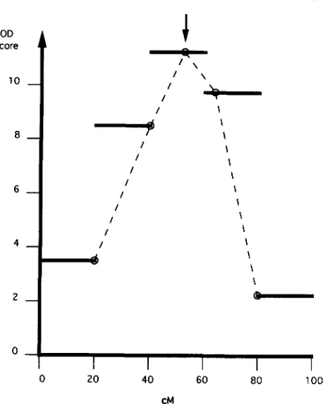
FIGURE 2.-Illustrative interval mapping example of results of a single simulation, with parameter values f l I = 0, p2 = 0.5, u = 1 , N

= 1000, c = 20 cM and the QTL located in the central interval at the mid-point between the two flanking markers. Maximum LOD scores within each interval are shown as horizontal bars, MLE of Q T L location within each interval shown as an open circle. Final estimate of map location of QTL (the estimate in the interval with the highest LOD score) shown by an inverted arrow.

TABLE 1

LOD score thresholds and type I errors

No. of markers

Marker _Per Per-marker LOD

interval chromosome type I error threshold

-0 -a2 _0.0026a ₁_.96a

10 11 0.0084 1.53

20 6 0.01 14 1.43

50 3 0.0171 1.19

Per-marker type I error, for the single-marker analysis, and LOD score threshold for the interval mapping analysis, as obtained from 10,000 replicate simulations, according to marker interval (in cM) in order to obtain a 0.05 per-chromosome type I error.

a Obtained from the expression of LANDER and BOTSTEIN (1989)

for an infinite number of markers.

0.5, u = 1 , N = 1000, c = 20 cM and the QTL located in the central interval, at the mid-point between the two flanking markers. T h e maximal LOD scores given by the various interval analyses are shown. On the basis of these LOD scores, the 40-60 CM interval was chosen to provide MLE of parameter values. T h e MLE of Q T L location is shown by the arrow.

Table 1 shows the per-marker type I error for the single marker analysis, and the LOD score thresholds used in the interval mapping analysis, for the various marker spacings. As expected, per-marker type I er-

Marker interval

500 t-test 0.66 0.61 0.64 0.68 0.58 0.58 0.71 0.50 0.47 (0.64) L R T 0.68 0.63 0.66 0.70 0.62 0.62 0.74 0.57 0.55

1000 t-test 0.94 0.94 0.91 0.95 0.90 0.88 0.95 0.83 0.75

(0.93) L R T 0.94 0.94 0.91 0.96 0.92 0.90 0.94 0.87 0.81

Power of detecting a Q T L with a standardized gene substitution effect of d = 0.25 in a 100-cM chromosome and with an overall per-chromosome type I error of 0.05, according to: marker interval (in cM); the relative location of the Q T L in the interval: 0, at the marker; %, half-way between the interval mid-point and the nearest marker; %, at the interval mid-point; N, the sample size; t-test, single-marker analysis using a t-test; LRT, interval mapping using a likelihood-ratio test. In parentheses under column headed “N,” power with an infinite number of markers.

a T h e relative location of the Q T L in the marker interval.

rors were lower, and LOD thresholds were higher for the narrower marker spacings.

Table 2 presents the power of detecting a QTL having standardized allele substitution effect d = 0.25 in a 100 cM chromosome, with a per-chromosome type I error of 0.05 (although included in the simulation, values are not given for a gene effect of d = 0.50 and N = 500, 1000, since in this case power was always close to 1.0). The power of the LRT for detecting a Q T L was the same for a spacing of IO cM as for infinite number of markers. Power was barely influenced by marker spacing in the range of 10 to 20 cM; e.g., for N = 500, the maximum difference in power between the 10 and 20 cM spacings, obtained when the QTL was midway between the two flanking markers (the worst case), was only 0.04. A somewhat greater difference was obtained when a 50 cM spacing was considered. In this case a maximum difference in power of 0.1 1 between 10- and 50-cM intervals was found; again, when the Q T L was at the mid-point of the interval. T h e difference in power according to marker spacing decreased when the Q T L was at a distance of ’/4 of the interval length from the nearest flanking marker.

T h e effect of using interval mapping with LRT as compared to single-marker analysis with a t-test was barely noticeable at marker spacings of 10 and 20 cM. For an interval of 50 cM and the Q T L located at the mid-point between the flanking markers, maximum power advantage of the LRT was found. Even then, it was only 0.08 and 0.06 for population sizes of 500 and 1000, respectively.

(5)

QTL Linkage Analysis 947

at all marker spacings. This is strictly correct when a single test is carried out, either LRT or t-test. How- ever, when several markers are tested, the specific number of markers included will influence the per- chromosome LOD score threshold, and hence the

per-marker type I error and power as well (Table 1). Consequently, when the Q T L is in absolute linkage to a marker, the power increases as fewer markers or intervals are scored. It is for this reason that when the QTL was at the marker

(k

= 0), the 50 cM spacing showed a higher power than the 10- or 20-cM spacing. Similarly, the LRT showed higher power than the t- test, because in the simulation the number of single markers was always one greater than the number of intervals (see Figure 1). This characteristic of complete marker-QTL linkage is mainly a simulation de- pendent artifact, since normally, in a marker-QTL linkage mapping exercise, there is a low probability that a QTL will be in absolute linkage to a scored marker. Some further aspects of this simulation be- havior will be considered in the DISCUSSION.

I n order to estimate the influence of allele substitution effect, d , and sample size,

N,

on the power of t-test and LRT for detecting a QTL, simulations with extended values of d (0.25, 0.5, 0.75, 1 .O, 1.5) and N

(100, 200, 500, 1000, 2000) were carried out for the representative case of marker intervals of 20 cM and the Q T L located at the mid-point

(k

= I/z) of the central marker interval. It was found that for all cases the difference in power between the two tests is small, with a common difference of 0.02 for most cases, and a maximal difference of 0.04.

T h e parameter estimates are expected to be asymp- totically unbiased since they are MLE. Indeed all the parameter estimates were as expected for simulations based o n 1000 replicates; bias was not found. There- fore, the standard errors of the parameter estimates are presented, rather than the estimates themselves. Although it was noted, when examining the individual simulations that interval mapping had a slight tendency to locate the QTL exactly at a scored marker, this did not cause a significant bias in the estimate of the Q T L map location.

Table 3 presents two estimates for the SE of the estimate of p I : (i) the empirical SE obtained from the 1000 replicate simulations for each parameter combination, (ii) the average of the SEE obtained from the covariance matrix at each individual simulation. Con- sideration of Table 3 shows that when using 10- or 20-CM spacings, the entire information on p , con- tained in the sample appears to be exploited, since the SE values obtained in the simulation are very close to the SE for the given population sizes for infinite number of markers (equal to 0.063 and 0.045 for

N

= 500 and 1000, respectively). For 50-cM spacing SE values increased slightly, to approximately 0.075 and 0.05 1 ,

respectively. T h e SEE obtained from the covariance matrix were unbiased estimators of the empirical SE for the 10- and 20-cM intervals. However, as compared to the empirical values, a slight bias upward (an average of 0.006) appeared at the 50-cM spacing. For

q2, the empirical SE and the SEE obtained from the covariance matrix for the MLE were both very small at all marker spacings (data not shown) so that this parameter was estimated with great accuracy at all marker spacings.

Table 4 presents the 95% confidence intervals for the QTL map location. T h e confidence interval was estimated in three different ways: (i) as an empirical 95% confidence interval obtained from the 1000 replicate simulations, (ii) as four times the empirical SE of the map location obtained from the 1000 replicate simulations, (iii) as four times the average, over the

1000 replicate simulations, of the SEE obtained from the covariance matrices. T h e first estimate is thought to be the most correct. T h e rationale for the last two estimates is that MLE are expected to be asymptoti- cally normally distributed. Consequently, 4 X SE would represent approximately the length of a 95% confidence interval. For the analysis based on an infinite number of markers, only empirical confidence intervals are presented. When required, the confidence interval calculated as 4 X SE or 4 X SEE was truncated at the chromosome length, 100 cM. T h e results summarized in Table 4 will now be considered in detail.

The influence of gene effect and population size on the empirical confidence interval for QTL loca- tion, with infinite number of markers: Even with an infinite number of markers, the confidence interval is strongly affected by population size and gene effect. Thus, with a population size of 500 and gene effect of 0.25, the empirical confidence interval for Q T L location with an infinite number of markers, was 90 cM. That is, the MLE placed the Q T L at more or less any location along the chromosome. In the parameter conditions studied, confidence interval, for infinite

number of markers was inversely proportional to population size and to the square of gene effect. Thus, for larger population sizes and/or greater gene effects, confidence interval with infinite markers decreased markedly, reaching, for example, 11 cM for a population size of 1000 and gene effect of 0.50. The dependence of confidence interval on population size and gene effect, even at infinite number of markers, shows that there is a limit confidence interval for map location. That is, increasing the number of markers can reduce the confidence interval only up to a given limit, which is determined by the size of the population and gene effect.

(6)

948 A. Darvasi et al.

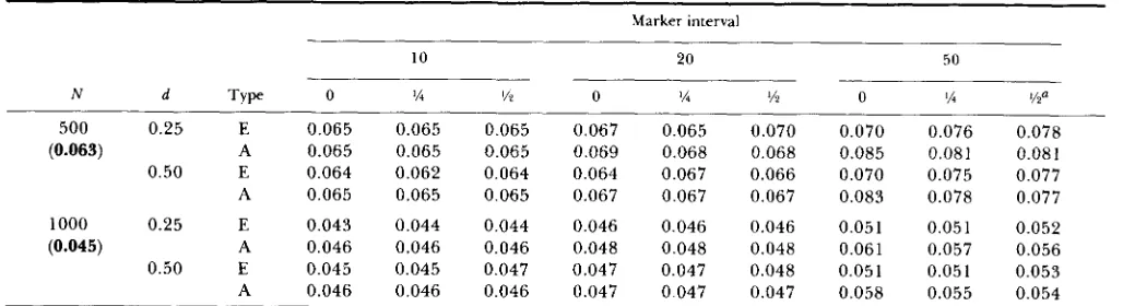
TABLE 3

Standard error of estimating QTL genotype mean

Marker interval

10 20 50

N d TY Pe 0 ‘A 1% 0 ‘/4 ’/2 0

‘/4

%a

500 0.25 E 0.065 0.065 0.065 0.067 0.065 0.070 0.070 0.076 0.078

(0.063) A 0.065 0.065 0.065 0.069 0.068 0.068 0.085 0.081 0.081

0.50 E 0.064 0.062 0.064 0.064 0.067 0.066 0.070 0.075 0.077

A 0.065 0.065 0.065 0.067 0.067 0.067 0.083 0.078 0.077

1000 0.25 E 0.043 0.044 0.044 0.046 0.046 0.046 0.051 0.051 0.052

(0.045) A 0.046 0.046 0.046 0.048 0.048 0.048 0.061 0.057 0.056

0.50 E 0.045 0.045 0.047 0.047 0.047 0.048 0.051 0.051 0.053

A 0.046 0.046 0.046 0.047 0.047 0.047 0.058 0.055 0.054

Standard errors of estimate of the mean of one of the Q T L genotypes according to standardized gene effect, d , and type of standard error: empirical SE (E), or average of the per simulation SEE estimated from the covariance matrix (A) (see text for details). Other headings as in Table 2. In parentheses, under column headed “N,” SE with an infinite number of markers.

a The relative location of the QTL in the marker interval.

TABLE 4

Confidence intervals for QTL map location

Marker interval

10 20 50

N d Type 50 47.5 45 40 45 50 50 37.5 25* 0 vi Yz 0 Y4 Yz 0 Y4 Y2Q

500 0.25 I 87 87 90 80 90 95 61 81 85

(90) E 67 73 73 66 77 81 65 89 100

A 29 30 28 88 49 54 100 100 100

0.50 I 14 22 25 17 3 1 37 36 60 50

(25) E 18 24 29 21 34 32 36 54 55

A 12 12 12 17 17 16 45 29 29

1000 0.25 1 49 55 63 40 55 59 45 65 73

(54) E 40 47 53 43 48 54 47 71 80

A 18 17 18 39 27 40 80 70 76 0.50 1 8 12 17 13 21 23 25 48 29

(11) E 10 12 15 12 19 21 24 42 32

A 8 8 8 11 12 12 27 18 17

The 95% empirical symmetric confidence interval for Q T L map location (in cM) obtained from 1000 replicate simulations for each parameter combination, (I) bold; and confidence intervals estimated as 4 X SE according to type of standard error: empirical SE, (E), or average of the per-simulation SEE obtained from the covariance matrix, (A). Other headings as in Tables 2 and 3. In parentheses in column headed “ d ” are 95% empirical SE obtained from 1000 replicate simulations for the case of infinite number of markers.

The relative location of the QTL in the marker interval. Distance of QTL from end of chromosome.

population size and gene effect: We first consider the effect of marker spacing on confidence interval for Q T L location, relative to confidence interval for infinite number of markers, for Q T L located at

K

=

‘/.I

(the average distance of a Q T L from its nearest

flanking marker). T h e effect of Q T L location relative to the flanking markers will be considered in the next section. Careful examination of Table 4 shows an interesting series of relationships.

For N = 500, d = 0.25, with a confidence interval

of 90 cM for an infinite number of markers, confidence intervals for marker spacing of 50, 20 and 10 cM were similar.

For N = 1000, d = 0.25, with a confidence interval of 54 cM for an infinite number of markers, confidence intervals for marker spacing of 50, 20 and 10 cM were again similar.

For N = 500, d = 0.5, with a confidence interval of 25 cM for an infinite number of markers, confidence intervals for marker spacing of 20 and 10 cM were less than for a marker spacing of 50 cM.

For N = 1000, d = 0.50, with a confidence interval of 11 cM for an infinite number of markers, the confidence interval for a marker spacing of 10 cM was markedly less than those for marker spacing of

20 or 50 cM.

T h e general impression from these results is that reducing marker spacing below the 95% confidence interval obtained with infinite markers did not add appreciably to narrowing the empirical confidence interval. This important result suggests that in practice, accuracy of estimation of QTL location will not be increased by decreasing marker spacing much beyond that equivalent to the 95% confidence interval obtained for an infinite number of markers. Now, as shown above, the confidence interval for an infinite number of markers is determined by the size of experiment and gene effect. Thus, these results suggest that the empirical 95% confidence interval appropriate to a given experimental design and estimated gene effect with infinite markers will give a rough estimate of the minimum useful marker spacing that can be expected to yield increments in the accuracy of estimation of QTL map location. This 95% confidence interval is obtained from the simulation results.

(7)

Q T L Linkage Analysis 949

( i e . ,

k

= 0 as compared to k = V4; or, k = '14 as

compared to

k

= I/z) the narrower the confidence interval. For example, for

N

= 1000 and d = 0.5, the confidence interval decreased from 17 cM at k = '12,

to 8 cM at k = 0. However, this general tendency was subject to a number of exceptions. In particular the confidence interval is influenced by the distance of the QTL from the end of the chromosome. Thus, confidence intervals, at the 50-cM marker spacing, were generally narrower for k = '/z than for k = '14.

This is due to the fact that the distance from the Q T L to the end of the chromosome differs according to QTL location relative to the markers (see heading of Table 4). This, in turn, places an upper limit on MLE error in the direction of the nearest chromosome end. For example, when the QTL is located 25 cM from the end of the chromosome, error in the distal direction is restricted to a maximum of 25 cM. Conse- quently, the confidence interval will be decreased relative to the situation where the QTL is located more centrally on the chromosome.

An additional simulation artifact relates to the ap- parent tendency of the interval mapping mode of analysis to locate the QTL at a marker. Consequently, for the interval mapping analysis, the confidence interval obtained, when the Q T L is assumed to be located at a marker, may be narrower than obtained when the simulation is based on an infinite number of markers! For example, at a 50 cM marker interval with

N

= 500 and d = 0.25, a value of 61 cM was obtained for the confidence interval with interval mapping. In this case only three markers are scored, two of which are at the chromosome extremes. Con- sequently, the estimated map location tends to be assigned to the central marker where the QTL is located. This dramatically reduces the confidence interval.

Confidence intervals based on empirical SE of QTL location and on SEE of the MLE of QTL loca- tion: 95% confidence intervals estimated as four times the empirical SE

(+2

SE) of QTL location, were generally quite close to the empirical confidence interval itself. This supports the expected normal distribution of the MLE, since the factor +2 SE determines a 95% confidence interval for a normal curve.

When the empirical confidence intervals were nar- row (1 0- 15 cM), the SEE estimates given by the covariance matrices of each simulation were close to the empirical confidence interval. They also did not differ much within each 1000-replicate simulation (data not shown). Thus, in this situation, utilization of Newton- Raphson procedure for MLE can provide useful SEE from the covariance matrix, for real experiments where only one replicate is available. When empirical confidence intervals were larger than this, however, the confidence interval estimated from the SEE often

diverged significantly from the empirical values, showing small confidence intervals. In this case they were also found to differ within each 1000-replicate simulation (data not shown). Thus, for such situations SEE obtained from the covariance matrices are not useful guides to the actual SE and confidence intervals. T h e small confidence intervals obtained from the SEE may derive from the fact that the profile likelihood for the map location is not smooth but increases within intervals and drops at the markers. T h e SEE considers the curve around the maximum which may be fairly peaked, but ignores the fact that outside the interval the surface may peak again.

DISCUSSION

Effect of population size, gene effect and marker spacing on power, SE of estimate of gene effects and confidence interval of QTL location: Increase in population size provided comparable gains in all three parameters of statistical importance: power, SE of estimate of gene effect, and confidence interval of Q T L location. Similarly, increase in gene effect provided comparable gains in all three of the above parameters. Furthermore, additional increase in population size or gene effect provided continuous additional im- provement in these statistical parameters. In contrast, the three statistical parameters were not uniformly affected by a reduction in marker spacing, and reduction in marker spacing did not have a continuous effect. In particular, with respect to power or SE of estimate of gene effect, marker spacing narrower than

10 or 20 cM did not provide additional gains, regard- less of the population size and gene effect. With respect to confidence interval of Q T L location, however, the marker spacing that provided information close to the resolving power of the experiment de- pended on the resolving power itself, as determined by gene effect and population size. Consequently, for mapping accuracy, 50-, 20-, 10-cM or even narrower marker spacing might be useful.

Confidence intervals for QTL map location: T h e results of theses simulations show that 95% confidence intervals for Q T L map location can be rather broad, in some cases essentially covering the entire chromosome. In effect, a Q T L with gene effect d = 0.25 in an experimental population of size 500 cannot be located with confidence to any particular region of the chromosome. For genes of large effect, however, or for experiments of greater size, confidence intervals can be considerably less, reaching, e.g., 11 cM for

(8)

increased accuracy of QTL mapping within a given experiment. Therefore, a priori it would appear reasonable to estimate the map resolution potential that a given experimental structure provides, and decide accordingly on the appropriate marker spacing to use. T o estimate this requires knowing the size of the experimental population and gene effect at the QTL, and then performing the corresponding simulation as previously described. T h e size of the experimental population is determined by experimental goals, facil- ities and resources. T h e gene effect at the QTL can be set according to a priori assumptions as to the magnitude of Q T L effect which it is desired to char- acterize; or can be estimated with relative accuracy by a preliminary experiment using a few widely spaced markers (see e.g., Table 3, 50-cM spacing). In practice extensive simulations are required in order to obtain the resolving power of the experiment. Consequently, for practical use, comprehensive tables showing confidence interval of Q T L in the infinite number of markers case, as a function of population size and gene effect for BC and F2 populations are in prepa- ration and will be published elsewhere.

Single-marker analysis as compared to interval mapping: In accord with results presented by HALEY and KNOTT (1 992), the difference in power between interval mapping using a LRT and single-marker analysis using a t-test was found to be small. When intervals of up to 20 cM are used, there will be little difference in the results obtained using the two methods. This differs from the conclusions of a previous study (LANDER and BOTSTEIN 1989) which suggested that power of detecting marker-QTL linkage could be markedly increased by utilizing interval mapping with LRT as compared to single markers with t-tests. This is probably due to the fact that the comparison previously investigated did not take into consideration that when a pair of flanking markers is available, both will be individually examined in the corresponding single-marker analysis. Statistical significance with respect to either will result in marker-QTL linkage identification, hence increasing the power of the single-marker analysis. Also, only the case where the QTL is located at the mid-point with respect to the flanking markers was investigated. This is the worst case for single-marker QTL linkage determination relative to interval mapping. Consequently, the increase in power given by interval mapping in relation to single-marker analysis which was found, was biased in favor of interval mapping.

Furthermore, as indicated above, in an initial screening of the genome for QTL detection, a rather wide marker spacing will be optimal. In practice, this means that the number of markers scored per chromosome will be one to three. In the case where one marker per chromosome is analyzed, it is obvious that

single-marker analysis should be used. When two markers are used they will be chosen to maximize power with respect to all possible QTL locations in the chromosome, ie., at a distance somewhat less than '14 from each chromosome end. Interval mapping can then be applied only to the single interval present, leaving the extremes unscreened. Therefore, in this case a single-marker analysis would be carried out in any event. Testing the single interval using interval mapping, in addition to the single-marker analysis, will cause a slight increase in the per-chromosome type I error. Alternatively, for the same per-chromosome type I error, power will slightly decrease. This will close the gap between the two methods and might even increase the power of the single-marker analysis as compared to interval mapping. T o a lesser extent, similar considerations will apply when three markers are scored on a chromosome.

T h e advantage of using single-marker analysis, as compared to interval mapping with LRT, lies in its simplicity. Single-marker analysis can be readily applied to any experimental design, and can be utilized for detection of several unlinked QTL using standard software packages for multiple regression (SAS, 1985), where QTL effects and their interaction can be simultaneously estimated. Also, when trait value is not normally distributed and its distribution is not known, the power of the LRT will decrease because the model in use is not an appropriate one. In contrast, by the Central Limit Theorem (MOOD, GRAYBILL and BOES 1974) the single-marker analysis will not be influenced by trait distribution for populations sizes generally studied ( N

>

100). In addition, single- marker analysis can be applied to unmapped markers, whereas, in interval mapping the markers must have been previously mapped, or sufficient markers and individuals should be scored to map the new markers as part of the same experiment.

T h e importance of interval mapping is in the second stage of the analysis, where an estimate of Q T L location is desired. In many cases the two stages will be implemented in different experimental populations, since detecting a QTL will require less effort than obtaining even an approximate gene location. There- fore, interval mapping will be essential only in experiments that are able to provide a fairly accurate gene location.

(9)

QTL Linkage Analysis 95 1

ments alone, even employing an “infinite number of markers” cannot bring Q T L mapping accuracy much beyond this point, for Q T L of moderate effect and experiments of acceptable size. One may conclude that fine mapping of Q T L will require other approaches, such as the use of near isogenic lines (BEN- TOLILA et al. 1991), recombinant congenic strains (DEMANT and HART 1986), substitution mapping (PA- TERSON et al. 1990) or backcross inbred lines (BECK- MANN and SOLLER 1989), all of which are based on definition of the chromosomal segment carrying a given QTL that is common to a number of individuals

or lines. Such approaches appear to hold the promise of providing effective means of utilizing the abun- dance of DNA-level markers for fine mapping of Q T L .

Selective genotyping (DARVASI and SOLLER 1992; LANDER and BOTSTEIN 1989; LEBOWITZ, SOLLER and BECKMANN 1987) was suggested as a design that can reduce the number of individuals genotyped for given power of detecting Q T L , by genotyping only the most informative individuals in the experimental population. T h e influence of selective genotyping on Q T L mapping accuracy remains to be investigated.

T h i s research was supported by the US.-Israel Agricultural Research and Development Fund (BARD). We thank ERIC LANDER for his counsel and encouragement in this and other studies.

LITERATURE CITED

BECKMANN, J. S., and M. SOLLER, 1989 Backcross inbred lines for mapping and cloning of loci of interest, pp. 1 17-122 in Devel- opment and Application of Molecular Markers to Problems in Plant Genetics, edited by B. BURR and T . HELENTJARIS. Brookhaven National Laboratory, New York.

BENTOLILA, S., C. CURTON, N. BOUVET, A. SAILAND, S. NYKAZA and G. FREYSSINET, 1991 Identification of an RFLP marker tightly linked to the H t l gene in maize. Theor. Appl. Genet. 82: 393-398.

DARVASI, A., and M. SOLLER, 1992 Selective genotyping for determination of linkage between a marker locus and a quantitative trait locus. Theor. Appl. Genet. 85: 353-359.

DEMANT, P., and A. M. HART, 1986 Recombinant congenic strains-a new tool for analyzing genetic traits determined by more than one gene. Immunogenetics 2 4 416-422.

DIXON, L. C., 1972 Nonlinear Optimization. The English Univer- sities Press, London.

EDWARDS, M. D., C. W. STUBER and J. F. WENDEL, 1987 Molecular-marker facilitated investigations of quantitative trait loci in maize. I . Numbers, genomic distribution and types of gene action. Genetics 116 113-125.

HALEY, C. S., and S. A. KNOTT, 1992 A simple regression method for mapping quantitative trait loci in line crosses using flanking markers. Heredity 69: 315-324.

J E N S E N ~ J . , 1989 Estimation of recombination parameters between a quantitative trait locus (QTL) and two marker gene loci. Theor. Appl. Genet. 78: 6 13-6 18.

KAHLER, A. L., and C. F. WEHRHAHN, 1986 Association between quantitative traits and enzyme loci in the F z population of a maize hybrid. Theor. Appl. Genet. 72: 15-26.

KNAPP, S. J., W. C. BRIDGES and D. BIRKES, 1990 Mapping quantitative trait loci using molecular marker linkage maps. Theor. Appl. Genet. 7 9 583-592.

LANDER, E. S., and D. BOTSTEIN, 1989 Mapping Mendelian factors underlying quantitative traits using RFLP linkage maps. Genetics 121: 185-199.

LEBOWITZ, R. J., M. SOLLER and J. S. BECKMANN, 1987 Trait- based analyses for the detection of linkage between marker loci and quantitative trait loci in crosses between inbred lines. Theor. Appl. Genet. 73: 556-562.

MOOD, A. M., F. A. GRAYBILL and D. C. BOES, 1974 Introduction

to the Theory ofStatistics. McGraw-Hill, New York.

NIENHUIS, J. T., T. HELENTJARIS, M. SLOCUM, B. RUGGERO and A. SCHAEFFER, 1987 Restriction fragment length polymorphism analysis of loci associated with insect resistance in tomato. Crop. Sci. 17: 797-803.

OSBORN, T . C., D. C. ALEXANDER and J. F. FOBES, 1987 Identification of restriction fragment length polymorphism linked to genes controlling soluble solids content in tomato fruits. Theor. Appl. Genet. 73: 350-356.

O n , J., 1985 Analysis of Human Genetic Linkage. John Hopkins Press, Baltimore.

PATERSON, A. H., E. S. LANDER, J. D. HEWITT, S. PETERSON, S. E. LINCOLN and S. D. TANKSLEY, 1988 Resolution of quantitative traits into Mendelian factors by using a complete linkage map of restriction fragment length polymorphisms. Nature

PATERSON, A. H., J. W. DEVERNA, B. LANINI and S. D. TANKSLEY, 1990 Fine mapping of quantitative trait loci using selected overlapping recombinant chromosome in an interspecies cross of tomato. Genetics 1 2 4 735-742.

SAS User’s Guide: Statistcs, Version 5, 1985. SAS Institute, Inc., Cary, N.C.

SAX, K., 1923 Association of size differences with seed-coat pat- tern and pigmentation in Phaseolus vulgaris. Genetics 8: 552- 560.

SIMPSON, S. P., 1989 Detection of linkage between quantitative trait loci and restriction fragment length polymorphisms using inbred lines. Theor. Appl. Genet. 77: 815-819.

SOLLER, M., T. BRODY and A. GENIZI, 1976 On the power of experimental designs for the detection of linkage between marker loci and quantitative loci in crosses between inbred lines. Theor. Appl. Genet. 47: 35-39.

SPICKETT, S. G., and J. M. THODAY, 1966 Regular responses to selection. 3 . Interaction between located polygenes. Genetic Res. 7: 96- 12 1.

THODAY, J. M . , 1961 Location of polygenes. Nature 191: 368- 370.

VAN OOIJEN, J. W., 1992 Accuracy of mapping quantitative trait loci in autogamous species. Theor. Appl. Genet. 84: 803-81 1. WELLER, J. I., 1987 Mapping and analysis of quantitative trait loci in Lycopersicon (tomato) with the aid of genetic markers using approximate maximum likelihood methods. Heredity 59: 41 3- 421.

WELLER, J. I . , M. SOLLER and T. BRODY, 1988 Linkage analysis of quantitative traits in an interspecific cross of tomato ( L ~ C O -

persicon esculentum X Lycopersicon pimpinellqolium) by means of genetic markers. Genetics 1 1 8 329-339.

335: 721-726.