Solving Stochastic and Bilevel Programs Using Value Functions of Integer Programs.

(1)

ABSTRACT

ZHANG, JUNLONG. Solving Stochastic and Bilevel Programs Using Value Functions of Integer Programs. (Under the direction of Osman Y. ¨Ozaltın.)

We employ value functions to optimize large-scale stochastic integer programs and

discrete bilevel programs. When solving such problems, many similar (bilevel) integer

programming (IP) subproblems are required to be solved. Optimizing these IP

subprob-lems directly one by one often consumes too much computing time. To overcome this

difficulty, we compute and store the value functions of integer programs in advance. In

the first part of this dissertation, we develop four efficient algorithms for computing the

value functions of single-ratio fractional integer programs (FIPs) based on properties such

as superadditivity and complementary slackness. These value functions are then used in a branch-and-bound algorithm to solve two-stage FIPs with stochastic right-hand sides.

The extensive forms of the instances solved in this part have a similar order of magnitude

to those of the largest stochastic quadratic integer programs solved in the literature. In

the second part, we propose a level-set characterization of the value functions of nonlinear

integer programs with nondecreasing integer-valued constraints. This characterization is

then exploited to optimize stochastic nonlinear integer programs with more constraints

compared to the stochastic FIPs addressed in the first part. In the third part, we extend

the above value function approach to solve discrete bilevel linear programs (DBLPs)

with binary upper-level variables and integer (or binary) lower-level variables. We de-rive structural properties of the value functions of bilevel integer programs and propose

three efficient approaches for computing them. These value functions are then employed

in a branch-and-cut solution algorithm enhanced with local search. The computational

results show that we can exactly solve DBLP instances with up to 200 variables and 150

(2)

(3)

Solving Stochastic and Bilevel Programs Using Value Functions of Integer Programs

by Junlong Zhang

A dissertation submitted to the Graduate Faculty of North Carolina State University

in partial fulfillment of the requirements for the Degree of

Doctor of Philosophy

Industrial Engineering

Raleigh, North Carolina

2018

APPROVED BY:

Yahya Fathi Shu-Cherng Fang

Michael Kay Andrew C. Trapp

External Member

(4)

DEDICATION

(5)

BIOGRAPHY

Junlong Zhang was born and grew up in Gulang, Gansu, China. In 2010, he received

his bachelor’s degree in Automation from Northwestern Polytechnical University, Xi’an,

Shaanxi, China. He then got enrolled and studied in a graduate program at the same

university. In 2011, he moved to the Hong Kong Polytechnic University to study for his

master’s degree in Transportation under the supervision of Prof. William H. K. Lam. In

(6)

ACKNOWLEDGEMENTS

I would like to thank my advisor Dr. Osman Y. ¨Ozaltın for his great guidance in my

research and also teaching during my Ph.D. study. He is a perfect example for me as a

rigorous and wise scholar. I also want to thank Prof. William H. K. Lam who is a great

supervisor and helped me a lot when I first started doing research in my master’s study.

I am very grateful to my committee members Dr. Yahya Fathi, Dr. Shu-Cherng Fang,

Dr. Michael Kay, and Dr. Andrew C. Trapp for their time and valuable comments on my Ph.D. work. Special thanks are given to Dr. Fang for his great support in my job

search process and his encouragement during my Ph.D. study. I also benefited a lot from

discussions with Dr. Trapp on my research. I also want to thank Dr. Gnanamanikam

Mahinthakumar (during prelim exam) and Dr. David Papp for agreeing to be my graduate

school representatives.

I also want to thank Dr. Maria Mayorga and Dr. Vanessa Doriott Anderson for their

guidance on my teaching. Many thanks to the staff in Department of Industrial & Systems

Engineering at NC State University, especially Ms. Cecilia Chen, Mr. Justin Lancaster

and Mr. Robert Lasson, for their help during my graduate study. I am also lucky to have many kind and helpful fellow labmates in rooms 373 and 375 in Daniels Hall at NC State

University.

Lastly but most importantly, I want to thank my parents and sisters for their

un-bounded love and unconditional support. Because of my busy graduate study and the

long distance, I was not able to spend much time with them in recent years. I really

regret that I was not there even when they needed me the most. After I graduate and

(7)

LIST OF TABLES

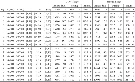
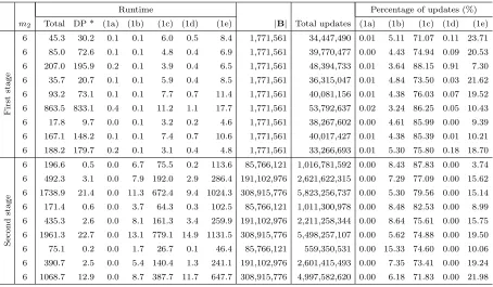
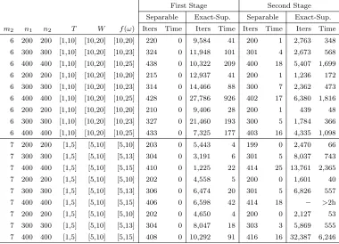
Table 2.1 Using the Exact-Superadditive Algorithm, the Sparse-Fixing Algorithm, and the Sparse-Enumeration Algorithm to construct the value functions of instances for which the denominator of the fractional objective is sparse. 30 Table 2.2 Runtime and number of updates of each step in the Exact-Superadditive

Algorithm when constructing the value functions of instances in

Ta-ble 2.1 with m2 = 6. . . 31

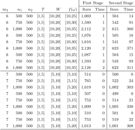
Table 2.3 Using the Sparse-Enumeration Algorithm to construct the value func-tions of large instances for which the denominator of the fractional objective is sparse. . . 32

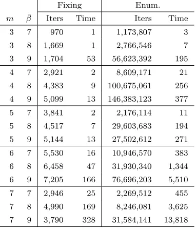
Table 2.4 The Sparse-Fixing Algorithm outperforms the Sparse-Enumeration Al-gorithm when (hT_x_{) has a small range and large domain. These FIP} instances are generated by setting each nonzero element of h to 1, and each column of the constraint matrixGcorresponding to a variable with a nonzero coefficient in hto a random 0-1 vector. All other nonzero el-ements of the G matrix are generated from the uniform distribution U[3,5]. In addition,a = 10,n = 200, and the elements of c, g,α and λ vectors are generated from the uniform distributionU[1,20]. The value function is characterized for allmdimensional right-hand sides between (0,0, . . . ,0)T _{and ( ¯}_β,_{β, . . . ,}_¯ _β_¯₎T_{. . . .} ₃₃

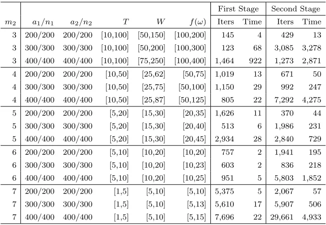
Table 2.5 Using the Exact-Superadditive Algorithm to construct the value func-tions of instances for which the denominator of the fractional objective function is not sparse, i.e., a1 =n1 and a2 =n2. . . 34

Table 2.6 Using the Separable-Fraction Algorithm and the Exact-Superadditive Algorithm to construct the value functions of instances with separable fractional objectives. . . 35

Table 2.7 Using the Separable-Fraction Algorithm to construct the value func-tions of large instances with separable fractional objectives. . . 36

Table 2.8 Using the branch-and-bound algorithm and the level-set approach to find an optimal right-hand side solution. . . 37

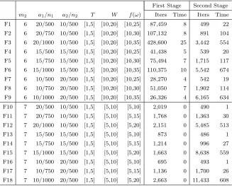
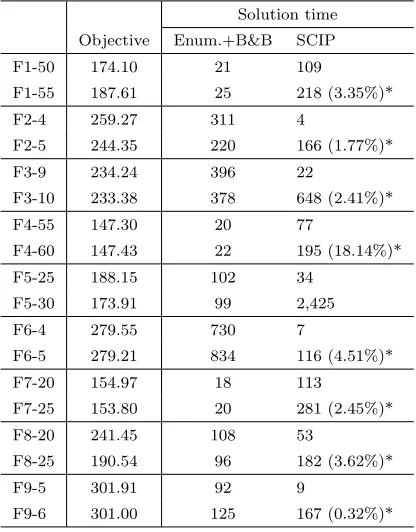
Table 2.9 Comparison between our two-phase approach and SCIP. . . 38

Table 3.1 Characteristics of test instances. . . 50

Table 3.2 Computational results. . . 52

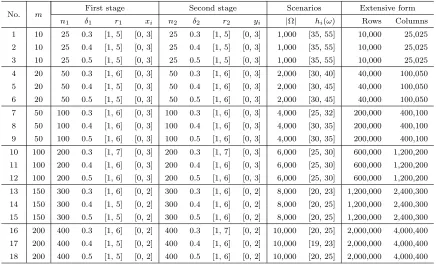
Table 4.1 Characteristics of instance classes in Testbeds 1 and 2. . . 74

Table 4.2 Characteristics of instance classes in Testbed 3. . . 74

Table 4.3 Computational results for instances in Testbed 1. . . 76

Table 4.4 Computational results for instances in Testbed 2. . . 76

(10)

(11)

Chapter 1 Introduction

Stochastic integer programs and discrete bilevel programs are important classes of

opti-mization problems with wide applications. They are nonetheless very difficult to solve.

The aim of this dissertation is to provide a value function solution approach for some

subclasses of these problems. In this chapter, we introduce the problems that are

ad-dressed in this dissertation, and our value function approach for solving them. We give the outline of this dissertation at the end of this chapter.

1.1 Stochastic integer programming

Stochastic programming [13, 70] models optimization problems that involve uncertainties

in the parameters. The probability distributions of the uncertain parameters are known

or can be estimated. A stochastic programming model is to find a solution that is feasible

for all (or almost all) possible realizations of the uncertain parameters and optimizes the

expectation of some function of the decision and the random variables.

Two-stage stochastic programs are the most widely applied and studied stochastic

programming models. In a two-stage stochastic program, part of the decisions are made

in the first stage before the uncertain parameters are realized. In the second stage, some

recourse actions can be taken as the actual values of the uncertain parameters are

re-vealed. The objective is to find first-stage decisions and a collection of second-stage

recourse decisions that optimize the deterministic first-stage cost plus the expected cost

of recourse actions taken in the second stage. We refer the readers to Zhang et al. [83] and

(12)

vechicle routing problems.

We focus on two-stage stochastic nonlinear integer programs as shown below:

(P1.1) : max f1(x) +_EωQ(x, ω) (1.1a)

subject to x∈_X⊂_Zn1_, _(1.1b)

where_Xis a finite set of first-stage feasible solutions, and_Eω is the expectation operator

with respect to the random variable ω. Given some x∈ _X and ω ∈ Ω, the second-stage problem is defined by the recourse function:

Q(x, ω) = max f2(y) (1.2a)

subject to W(y)≤h(ω)−T(x), (1.2b)

y ∈_Y⊂_Zn2_, _(1.2c)

where _Y is a finite set of second-stage feasible solutions.

In (P1.1), the number of decision variables in stage i is ni, for i = 1,2. Functions

f1(·) : _Zn1 _7→

R, f2(·) : Zn2 7→ R, W(·) : Zn2 7→ Rm and T(·) : Zn1 7→ Rm can be nonlinear. The random variable ω ∈Ω is assumed to follow a discrete distribution with finite support. This assumption is justified by Schultz [67], who showed that the optimal

solution to a stochastic program with continuously distributed ω can be approximated within any desired accuracy using a discrete distribution. The realizations of the uncertain

right-hand side vectorh(ω)∈_Rm _{in the second-stage problem are referred to as}_scenarios_. Note that h(ω) is the only stochastic component in (P1.1) and other parameters are deterministic. We also assume thatQ(x, ω) is finite for allx∈_X and ω ∈Ω.

Two-stage stochastic nonlinear integer programs with discrete variables in the second

stage are particularly difficult to solve because of the discontinuity and nonconvexity of

the expected recourse function [13]. Standard convex programming approaches that work for stochastic linear programs can not be employed for solving (P1.1). In the literature, algorithms developed for solving stochastic programs with integer recourse utilize cutting

planes and/or column generation techniques in combination with decomposition methods

that exploit block-separability of the underlying problem structure. Here we describe

the papers that are most closely related to our work (for general reviews of stochastic

programming, see [13, 68, 70]).

(13)

first stage and pure-integer second stage. They apply a variable transformation to make

the discontinuities of the expected recourse function orthogonal to the variable axes. This

structure is then exploited through a hyper-rectangular branching strategy that isolates

discontinuous pieces. A bounding strategy is applied to construct the value function of the

second-stage integer program in the absence of discontinuities. Finiteness of the method

is established as there is only a finite number of discontinuous pieces of the value function.

Kong et al. [50] considers two-stage stochastic linear programs with pure-integer

first-and second-stage problems. In their model, the uncertainty can only appear in the

right-hand sides of the second-stage problem. Therefore, Kong et al. [50]’s model is a special

case of (P1.1). Similar to Ahmed et al. [1], the solution approach of Kong et al. [50] is based on a variable transformation. The value functions of both stages are computed

in advance, and then utilized in a global branch-and-bound algorithm or an implicit

exhaustive search method. Superadditive duality properties of linear integer programs

are derived and used to construct value functions efficiently. ¨Ozaltın et al. [61] extends

the solution approach of Kong et al. [50] to two-stage quadratic integer programs with

stochastic right-hand sides. They derive superadditivity and complementary slackness

properties for the value functions of quadratic integer programs.

Trapp et al. [74] shows that the value function of a pure integer linear program can be

characterized entirely by its values on the set of right-hand side vectors that are minimal with respect to their objective function level set. Since the number of the level-set minimal

right-hand sides that can be generated by nonnegative integer linear combinations of the

columns of the first-stage constraint matrix is generally much smaller than that of the

entire set of feasible first-stage right-hand sides, the memory requirements to store the

value functions can be greatly reduced. Trapp et al. [74] also extends the global

branch-and-bound algorithm of Kong et al. [50] to search over the level-set minimal right-hand

sides.

In this dissertation, we solve two important subclasses of (P1.1) using value func-tions of nonlinear integer programs. The first is a class of single-ratio fractional integer programs (FIPs) with stochastic right-hand sides, in which the objective functions f1₍_·₎

and f2₍_·_{) are single-ratio FIPs and the constraint functions} _W₍_·_{) and} _T₍_·_{) are linear.}

We reformulate the problem using the value functions of the first- and second-stage

FIPs. To solve this reformulation, we first compute the value functions, and then use a

(14)

pro-posed method is that it is relatively insensitive to the number of variables and scenarios.

However, the number of right-hand sides that must be considered when constructing the

value functions grows exponentially in the number of constraints. A major contribution

of this dissertation is developing algorithms that can mitigate the effect of this

exponen-tial growth to some extent by exploiting the properties of the value functions of FIPs.

We show that our approach can solve instances that have up to seven constraints in

each stage. Extensive forms of these instances have the same size as the largest two-stage

stochastic quadratic [61] integer programs solved in the literature.

We then turn to a class of more general two-stage nonlinear integer programs with

stochastic right-hand sides, in whichf1(·) and f2(·) can be nonlinear, andW(·) and T(·) are nondecreasing and integer-valued (nonlinear) functions. To apply the above value

function approach, we need to compute the the value function of a nonlinear integer

pro-gram with nondecreasing integer-valued constraints. Properties such as superadditivity

and complementary slackness, however, do not hold in general for such value functions.

Instead, we extend the level-set minimal concept introduced by Trapp et al. [74] to the

nonlinear case we consider at this stage and propose a level-set characterization of such

value functions. This characterization is then exploited in a global branch-and-bound

algorithm to optimize more general stochastic nonlinear integer programs with a greater

number of constraints compared to the stochastic FIPs addressed above.

1.2 Discrete bilevel programming

We further extend the value function approach described in Section 1.1 to solve a class

of discrete bilevel linear programs. Bilevel programs [6, 29, 32] model the hierarchical

relationship between two autonomous and possibly conflicting decision makers: theleader

and thefollower. Each decision maker controls a distinct set of variables and the decisions are made sequentially according to a hierarchy: the upper-level decisions are made first by the leader, after which the lower-level decisions are made by the follower subject to

constraints which depend on the leader’s decisions. The follower’s decisions in return

affect the leader’s objective function. Thus, the leader should act by considering the

follower’s response.

Bilevel programming is closely related to the static Stackelberg leader-follower game [22,

(15)

decentralized decision-making in several important application domains including

haz-ardous material transportation [42], network design [27, 71], revenue management [30],

traffic planning [55, 62], energy [9], computational biology [20, 65] and defense [19] areas.

In this dissertation, we consider the following discrete bilevel linear programs (DBLPs)

where the upper-level variables are binary and the lower-level variables are either pure

integer or pure binary:

(P1.2) : max cTx+dTy (1.3a)

subject to x∈_Bn1_, _(1.3b)

y∈argmaxtTy | Ay≤b−Bx, y ∈_Y , (1.3c)

where x and y represent the leader’s and the follower’s decision variables, respectively, and A and B are m2×n2 and m2×n1 constraint matrices. The discrete set Y restricts

the follower’s variables to be pure binary or pure integer.

We propose a finite branch-and-cut (B&C) algorithm as an exact solution method

for solving (P1.2). To avoid repeatedly solving similar lower-level problems for different upper-level solutions in the B&C algorithm, we study the properties of the value

func-tions of bilevel integer programs. Most notably, we generalize the integer complementary

slackness theorem to bilevel integer programs. We also propose three efficient approaches

for computing the bilevel programming value functions. These value functions are then

utilized when calculating bounds in the B&C algorithm.

Any linear mixed 0–1 programming problem can be reduced to a bilevel linear program

(BLP), in which the leader’s and the follower’s problems are both linear programs [5].

Therefore, BLPs, and so DBLPs and bilevel programs in general, are strongly N P -hard [43]. For BLPs, Bard and Moore [7] proposed a branch-and-bound algorithm that branches on complementarity conditions. Hansen et al. [43] extended this algorithm by

exploiting the necessary optimality conditions of the follower’s problem. Another

ap-proach by J´udice and Faustino [47] used complementary pivoting to achieve -optimal solutions. We refer the reader to Ben-Ayed [11] for a detailed survey on BLPs.

For mixed-integer bilevel programs (BMIPs) including mixed-integer linear programs

in the upper and lower levels, Moore and Bard [58] proposed a branch-and-bound

algo-rithm. DeNegre [35] improved this algorithm using cutting planes. Lozano and Smith [52]

(16)

on value function reformulation. Vicente et al. [75] used penalty functions to reformulate

BMIPs into bilinear programs. Audet et al. [5], Dempe [31] and Wen and Yang [77]

pro-posed solution approaches for specific classes of BMIPs where either the leader’s or the

follower’s variables are all continuous. Dempe and Richter [34], ¨Ozaltın et al. [60] and

Brotcorne et al. [18] considered the bilevel knapsack problem, an extension of the

classi-cal knapsack problem to the bilevel framework. Detailed surveys on bilevel programming

solution techniques were presented in [6, 32, 56].

We review below previous work in the literature that is closely related to (P1.2). Bard and Moore [8] studied bilevel programs with binary upper- and lower-level variables. They

proposed an algorithm that implicitly enumerates the upper-level variables and solves the associated lower-level problems to obtain bilevel feasible solutions. The authors reported

solving instances with up to 45 variables and 18 constraints. Caramia and Mari [24] and

DeNegre and Ralphs [36] studied bilevel integer programs (BIPs) with integer

upper-and lower-level variables. They derived valid inequalities to eliminate bilevel-infeasible

solutions for a given upper-level solution in a branch-and-bound framework. Caramia

and Mari [24] reported solving BIPs with up to 25 variables and 25 constraints, while

DeNegre and Ralphs [36] performed tests using a set of interdiction problems with up to

34 variables and 19 constraints. Zeng and An [82] proposed a single-level reformulation

for BMIPs by enforcing the optimality conditions for the continuous variables for each fixed value of the integer variables in the lower-level problem. They offered a

column-and-constraint generation algorithm to solve this reformulation. The authors reported solving

pure integer instances with up to 20 variables and 30 constraints. Dempe and Kue [33] also

studied BIPs in which upper-level variables only affect the lower-level objective function.

The authors proposed a B&C algorithm based on an optimal value reformulation of the

follower’s problem and presented small illustrative examples.

Our proposed solution approach differs from the existing methods in the literature

because we utilize value functions of BIPs in our B&C algorithm to avoid repeatedly

solving similar lower-level problems. In addition, we implement local search to find im-proved bilevel-feasible solutions. Finally, we strengthen the relaxed node subproblems in

the B&C algorithm by generating cuts to eliminate all of the upper-level integer

feasi-ble solutions explored during the local search step. Our numerical results show that the

proposed B&C algorithm enhanced with the implementation of value functions and local

(17)

a reasonable amount of time.

1.3 Value functions of integer programs

Value functions of integer programs are key components in our value function solution

approach. Given G ∈ _Rm×n _and _γ _∈

Rn, consider the family of parameterized linear integer programs:

(PIP) : ζ(β) = max{γT_x _| _x_∈_S₍_β₎_{}, S}₍_β_{) =}_{x_∈

Zn+ | Gx≤β}, forβ ∈Zm.

The function, ζ(·) : _Zm _7→

R, is called the value function of (PIP). Define optc(β) =

argmax{γT_x_| _x_∈_S₍_β₎_}_{. Denote the} _jth _{column of matrix}_G _by_G

j, and the jth element of vector γ byγj.

Proposition 1. The following results are compiled in Nemhauser and Wolsey [59]. (1) ζ(Gj) ≥ γj for j = 1, . . . , n. If ζ(Gj) > γj, then xˆj = 0 for all β ∈ Zm and

ˆ

x∈optc(β).

(2) ζ(·) is nondecreasing in β ∈_Zm_.

(3) ζ(·) is superadditive over D={β ∈_Zm _| _S₍_β₎₆₌_∅}_.

(4) ζ(0)∈ {0,∞}. Ifζ(0) =∞, thenζ(β) =±∞ ∀β∈_Zm_{. If}_ζ₍₀_{) = 0}_{, then}_ζ₍_β₎_<_∞

∀β ∈_Zm_.

(5) (Integer Complementary Slackness) If xˆ∈optc(β), then ζ(Gx) =γTx and ζ(Gx) +

ζ(β−Gx) = ζ(Gx) +ζ(G(ˆx−x)) = ζ(β), for all x∈_Zn

+ such that x≤xˆ.

Value functions of integer programs play a central role in classical duality theory [14,

15, 41, 78], and they are also critical elements of solution methods for important classes

of optimization problems such as stochastic integer programs [1, 50, 61, 74] and bilevel

integer programs [52]. Most of the previous work on value functions focus on the linear

case [15, 50, 78]. One work of particular interest is by Trapp et al. [74], who showed

that the value function of a pure integer linear program can be characterized entirely by

its values on the set of right-hand side vectors that are minimal with respect to their

(18)

generally difficult to verify, the authors proposed a larger set that contains all level-set

minimal vectors. This larger set can be constructed in a straightforward manner and yet

maintains many of the desirable properties of the level-set minimal vectors.

In this dissertation, we study properties of value functions of nonlinear integer

pro-grams and design efficient algorithms for computing these value functions. We utilize

these value functions in solving stochastic nonlinear integer programs described in

Sec-tion 1.1. We also investigate value funcSec-tions of bilevel integer programs, which are then

used in our value function approach for solving (P1.2).

1.4 Outline of the dissertation

The rest of this dissertation is organized as follows. In Chapter 2, we present our value

function solution approach for a class of single-ratio fractional integer programs with

stochastic right-hand sides. In Chapter 3, we propose a level-set characterization of the

value functions of nonlinear integer programs with nondecreasing integer-valued

con-straints. We exploit this characterization to optimize more general stochastic nonlinear

integer programs than those addressed in Chapter 2. In Chapter 4, we extend the value

function approach to solve discrete bilevel linear programs with binary upper-level vari-ables and integer (or binary) lower-level varivari-ables. In Chapter 5, we summarize our work

(19)

Chapter 2 Two-Stage Fractional Integer

Programs with Stochastic

Right-Hand Sides

We present an equivalent value function reformulation for a class of single-ratio fractional

integer programs (FIPs) with stochastic right-hand sides, and propose a two-phase

solu-tion approach. The first phase constructs the value funcsolu-tions of FIPs in both stages. The

second phase solves the reformulation using a global branch-and-bound algorithm or a

level-set approach. We derive some basic properties of the value functions of FIPs and

utilize them in our algorithms. We show that in certain cases our approach can solve

in-stances whose extensive forms have the same order of magnitude as the largest stochastic

quadratic integer programs solved in the literature.

2.1 Introduction

We consider the following class of two-stage fractional integer programs (FIPs) with

stochastic right-hand sides:

(P2.1) : max cTx−g

T

1x+α1 hT

1x+λ1

+_EωQ(x, ω) (2.1a)

(20)

where _X={x∈_Zn1

+ |Ax ≤`} is a finite set of first-stage feasible solutions and,

Q(x, ω) = max dTy(ω)− g

T

2y(ω) +α2 hT

2y(ω) +λ2

(2.2a)

subject to W y(ω)≤f(ω)−T x, (2.2b)

y(ω)∈_Zn2

+. (2.2c)

The numbers of constraints and decision variables in stage i are mi and ni, respec-tively, for i = 1,2. We assume that a/0 = +∞ if a > 0 and a/0 = −∞ if a < 0. The random variable ω ∈ Ω follows a discrete distribution with finite support and de-scribes the realizations of the uncertain right-hand side vector f(ω) ∈ _Rm2_{, referred to}

as scenarios. Other parameters in (P2.1) are deterministic and their values are known with certainty. We assume that the first-stage constraint matrix A, technology matrix

T, and recourse matrix W are all integral, i.e., A ∈ _Zm1×n1_, _T _∈

Zm2×n1, W ∈ Zm2×n2. This assumption is not overly restrictive in a sense, as any rational matrix can be

con-verted to an integral one. Without loss of generality, we also assume that ` ∈ _Zm1 _and f(ω)∈_Zm2 ∀ω∈_{Ω, as} _{A, T}_{, and} _W _{are all integer.}

When all decision variables are continuous, a single-ratio fractional program can be

reformulated as a linear program through Charnes and Cooper’s transformation [25]. In

(P2.1), however, all decision variables are integers giving rise to nonconvex problems in both stages. Note that FIPs generalize 0-1 fractional programs [16], which are

ex-tensively studied in the literature [51, 63, 66, 73, 80]. There is a variety of real-world

applications of FIPs and 0-1 fractional programs in bin packing [57], resource

alloca-tion [2], scheduling [81], producalloca-tion [28], wireless network design [3], biclustering [21],

revenue management [17], and facility location [12].

We motivate the problem studied in this chapter by providing a specific application

of single-ratio FIPs with stochastic right-hand sides. Consider the customer allocation

problem of a firm facing demand uncertainty. The firm has already investedf > 0 dollars to set up service facilities j ∈ J. Its objective now is to maximize the expected value of the profitability index – the ratio of total profit to total cost [10]. A discrete set

of scenarios is considered with a given probability distribution, where dω

i denotes the demand at customer location i under scenario ω ∈ Ω. Integer decision variable y_ijω ≥ 0 denotes the demand at customer location i that is allocated to facility j under scenario

(21)

formulation is given by:

max

(

Eω

" _P

i∈I

P

j∈Jrijy ω ij

f+P

i∈I

P

j∈Jcijy ω ij # X

j∈J

y_ijω ≤dω_i, yω_ij ∈_Z+, i∈I, j ∈J, ω ∈Ω

)

.

(2.3)

Problem (2.3) is an instance of (P2.1). Our goal in this chapter, however, is to investigate the structural properties of the generic problem (P2.1) and develop efficient solution algorithms.

We reformulate (P2.1) using the value functions of the first- and second-stage FIPs. To solve this reformulation, we first compute the value functions, and then use a global

branch-and-bound algorithm or a level-set approach. The advantage of the proposed

method is that it is relatively insensitive to the number of variables and scenarios.

How-ever, the number of right-hand sides that must be considered when constructing the

value functions grows exponentially in the number of constraints. A major contribution

of this chapter is developing algorithms that can mitigate the effect of this exponential

growth to some extent by exploiting the properties of the value functions of FIPs. We

show that our approach can solve instances of (P2.1) that have up to seven constraints in each stage. Extensive forms of these instances have the same size as the largest two-stage stochastic quadratic [61] integer programs solved in the literature.

The remainder of this chapter is organized as follows. Section 2.2 presents an

equiva-lent reformulation of (P2.1) using value functions. Section 2.3 develops a global branch-and-bound algorithm and a level-set approach to optimize this reformulation. Section 2.4

derives some properties of the value functions of FIPs that are subsequently used in our

algorithms in Section 2.5 for efficient construction of value functions. Section 2.6

dis-cusses the details of our implementation and computational results. Finally, Section 2.7

presents a summary of this chapter.

2.2 Value function reformulation

We reformulate (P2.1) using the value functions of FIPs in both stages. Let B1 _be

the set of vectors β1 ∈ Zm2 such that there exists a first-stage solution x ∈ X ⊂ Zn+1

(22)

B2 ₌S

β1∈B1∪ω∈Ω{f(ω)−β1}.

Note that B1 _and _B2 _{are finite sets since}

X and Ω are finite. For any β1 ∈Zm2, the first-stage value function of (P2.1) is defined as:

ψ(β1) = max

cTx−g

T

1x+α1 hT

1x+λ1

| x∈S1(β1)

, S1(β1) ={x∈X | T x≤β1}. (2.4)

Similarly, for any β2 ∈_Zm2_{, the second-stage value function of (}_P₂_._{1) is defined as:}

φ(β2) = max

dTy− g

T

2y+α2 hT

2y+λ2

| y∈S2(β2)

, S2(β2) =y∈_Zn2

+ | W y ≤β2 . (2.5)

The value function reformulation of (P2.1) obtained by using ψ(·) and φ(·) is then given by:

(P2.2) : maxψ(β) +_Eωφ(f(ω)−β) | β ∈B1 . (2.6) The variablesβin (P2.2) are known as thetender variables [1, 50, 61]. Instead of searching over _X, we search over the set B1 _{of tender variables to optimize (}_P₂_._{2). Theorem 1}

establishes the relationship between the optimal solutions to (P2.1) and (P2.2).

Theorem 1. Letβ∗ be an optimal solution to(P2.2). Then,x∗ ∈argmaxcT_x₋g1Tx+α1

hT 1x+λ1 | x∈S1(β∗) is an optimal solution to (P2.1). Furthermore, the optimal values of the two

problems are equal.

The proof of Theorem 1 is similar to Theorem 2 in Ahmed et al. [1]. Section 2.3

presents a global branch-and-bound algorithm and a level-set approach to optimize (P2.2) over the setB1 of tender variables given the value functions of FIPs in both stages. These two methods motivate us to derive some basic properties of the FIP value function in

Section 2.4. The derived properties are then utilized in our algorithms for constructing

the value functions of FIPs in Section 2.5.

2.3 Finding the optimal tender

(23)

2.3.1 A global branch-and-bound algorithm

We derive a global branch-and-bound algorithm [44], which partitions B1 _into

hyper-rectangles Pk_{. For each hyper-rectangle} _Pk_{, we have an associated subproblem of the}

form:

fk = maxψ(β) +_Eωφ(f(ω)−β) |β ∈ Pk _(2.7)

We do not solve subproblem (2.7) exactly, but instead generate a lower bound µk _≤_fk_, and an upper bound vk _≥ _fk_{. Let} _L _{be the incumbent solution’s objective value. A} hyper-rectangle Pk _{is fathomed by feasibility if} _µk ₌ _vk_{, or by bound if} _vk _≤ _L_{, or by} infeasibility if Pk_∩_B1 ₌_∅_{. The list of unfathomed hyper-rectangles is denoted by} _M_.

Algorithm 2.1. A global branch-and-bound algorithm to solve (P2.2).

Step 0: (Initialization)SinceB1 is a finite set, there exists a hyper-rectangleP0 _:=

[λ0, η0] = Πm2

i=1[λ0i, ηi0] such that B1 ⊆ P0 ∩Zm2. Initialize list M ← {P0} and

k ← 1. Set global lower bound L = ψ(β0) +_Eωφ(f(ω)−β0) using an arbitrary

β0 _∈ _B1_{. Set the lower and upper bounds for} _f0 _as _µ0 ₌ _ψ₍_λ0_{) +}

Eωφ(f(ω)−η0) and v0 ₌_ψ₍_η0_{) +}

Eωφ(f(ω)−λ0), respectively.

Step 1: (Subproblem selection) If M = ∅, terminate with optimal solution β∗; otherwise, select and delete fromMa hyper-rectanglePk _:=

λk_{, η}k

= Πm2

i=1

λk i, ηki

.

Step 2: (Subproblem pruning)

(2a) Ifvk ≤L orPk_∩_B1 ₌_∅_{, go to Step 1.}

(2b) Ifµk< vk, i.e. Pk _{is an unfathomed hyper-rectangle, go to Step 3.}

(2c) Ifµk ₌_vk_and_{L < µ}k_{, update}_L₌_µk₌_vk ₌_fk_{, and select}_β∗ ₌_β_{∈ P}k_∩B1_.

(2d) Delete fromM all hyper-rectanglesPk0 _with _vk0 _≤_L_{and go to Step 1.}

Step 3: (Subproblem partitioning) Choose a dimension i0,1 ≤ i0 ≤ m2, such

that λk

i0 < η_ik0. Divide Pk into two hyper-rectangles Pk1 and Pk2 along

dimen-sion i0 as: Pk1 _:= _λk1_{, η}k1 ₌ _λk

i0,b(ηki0 +λk_i0)/2c

× Πi6=i0λk

i, ηik

and Pk2 _:=

λk2_{, η}k2 ₌ _b₍_ηk

i0+λk_i0)/2c+ 1, ηk_i0

× Πi6=i0λk_i, η_ik. Set M ← M ∪Pk1,Pk2 .

Set µki ₌ _ψ₍_λki_{) +}

(24)

Theorem 2. [50] Algorithm 2.1 terminates with an optimal solution β∗ to (P2.2) after a finite number of iterations.

Algorithm 2.1 requires the first-stage value functionψ(·) overP0 _{and the second-stage}

value functionφ(·) over the set of right-hand sides induced byP0_{. Note that}_λk_≤_β _≤_ηk for allβ ∈ Pk_{. The lower bound}_µk_{and the upper bound}_vk_{follow from the nondecreasing} property of ψ(·) andφ(·), i.e. ψ(λk₎_≤_ψ₍_β₎_≤_ψ₍_ηk_{) and} _φ₍_f₍_ω₎₋_ηk₎_≤_φ₍_f₍_ω₎₋_β₎_≤

φ(f(ω)− λk_{) for all} _ω _∈ _{Ω. Rules used in Step 1 (subproblem selection) and Step 3} (subproblem partitioning) as well as the method employed for generating the initial

global lower bound affect the performance of the B&B algorithm significantly. Although

the best approach is problem-specific, efficient rules can be found through computational

experiments. In our implementation, the hyper-rectangle that has the smallest upper

bound is selected in Step 1. In Step 3, the dimension that has the largest range, i.e.,

i0 ∈ argmax{(ηk_i −λk_i) | i ∈ {1, . . . , m2}}, is selected for branching. The initial global

lower bound is set to the maximum objective value of (P2.2) with respect to 0 and b1, i.e., max{ψ(0) +_Eωφ(f(ω)), ψ(b1) +Eωφ(f(ω)−b1)}, where b1 is the largest vector in

B1 _{componentwise.}

2.3.2 A level-set approach

We develop a level-set approach when T matrix is nonnegative so that B1 ⊂ _Zm2 + . In

this case, there must be an optimal right-hand side β∗ to (P2.2) satisfying the condition that each smaller right-hand side has also a strictly smaller objective value in the first

stage. This approach is first introduced in Kong et al. [50] for two-stage stochastic linear integer programs, and then generalized in Trapp et al. [74] by relaxing the restrictions

on the sign of T matrix.

A vectorβ ∈B1 _{is a}_{minimal tender} _if_β

i = 0 orψ(β−ei)< ψ(β) for alli= 1, . . . , m2,

where ei is the ith unit vector. Let Θ⊆B1 be the set of all minimal tenders.

Theorem 3. There exists an optimal solution to (P2.2) that is a minimal tender, that is

max

β∈Θ {ψ(β) +Eωφ(f(ω)−β)}= maxβ∈B1{ψ(β) +Eωφ(f(ω)−β)}.

(25)

lexicographically minimum optimal tender. Then there exists i ∈ {1, . . . , m2} such that β_i ≥1 and ψ(β−ei) =ψ(β). Sinceφ(·) is nondecreasing (see Remark 2 in Section 2.4), for anyω∈Ω,φ(f(ω)−β)≤φ(f(ω)−(β−ei)). Henceψ(β−ei) +Eωφ(f(ω)−(β−ei))≥

ψ(β) +_Eωφ(f(ω)−β). This indicates thatβ−ei is an optimal tender in (P2.2), which contradicts the fact that β is the lexicographically minimum optimal tender.

Letρ=|Θ|/|B1_|_{. Intuitively, as} _ρ_→_{1, the computational benefit of searching Θ may}

be surpassed by the computational burden of determining Θ. The value ofρ, however, is usually unknown unless ψ(·) is completely determined.

Remark 1. Letopt(β)⊆_Zn1

+ denote the set of optimal solutions toψ(β). For any β∈Θ

and xˆ∈opt(β), Txˆ=β.

Remark 1 is intuitive because if Txˆ 6= β, then ψ(β) = ψ(Txˆ) and Txˆ ≤ β, which means that β is not a minimal tender.

Proposition 2. Let xˆ∈opt(β) and column vector g1 = 0. If β ∈Θ, then T x∈Θ for all x≤xˆ such that hT₁(ˆx−x) = 0.

Proof. Let x ≤ xˆ be such that hT_(ˆ_x₋_x_{) = 0. Then} _ψ₍_{T x}₎ _≥ _cT_x₋ α1

hT

1x+λ1. Suppose

that T x /∈ Θ. Then there exists an i ∈ {1, . . . , m2} such that ψ(T x−ei) = ψ(T x). Let

y∈opt(T x−ei). Thusy6=x,y∈S1(T x−ei) andcTy−_hTα1

1y+λ1 =ψ(T x)≥c

T_x₋ α1

hT 1x+λ1.

Consider ˜x= ˆx−x+y. Then Tx˜ =T(ˆx−x+y)≤Txˆ−T x+T x−ei =Txˆ−ei and ˜

x∈S1(Txˆ−ei). The objective value for ˜x:

cT(ˆx−x+y)− α1 hT

1(ˆx−x+y) +λ1

=cT(ˆx−x) +cTy− α1 hT

1y+λ1 ,

≥cT(ˆx−x) +cTx− α1 hT

1x+λ1

=cTxˆ− α1 hT

1xˆ+λ1 ,

which implies that ψ(Txˆ−ei) =ψ(Txˆ) contradictingTxˆ=β ∈Θ.

Proposition 2 applies to linear integer programs sincehT₁(ˆx−x) = 0 for allx≤xˆwhen

h1 = 0. For linear integer programs, Kong et al. [50] showed that for any β∈Θ\ {0}and ˆ

x∈opt(β), if ˆx` ≥1, thent`∈Θ, where t` is the`thcolumn ofT, whenT is nonnegative. However, Kong et al.’s [50] result does not hold for FIPs. Consider the following instance:

z(β) = max

x1−x2− 4 x2+ 1

| 2x1+x2 ≤β1, 2x1+ 2x2 ≤β2, x∈_Z2₊

(26)

Note that ˆx= (1,1)T _∈_opt₍₍₃_,₄₎T_{) and}_z₍₍₃_,₄₎T_{) =} ₋_{2. Furthermore, (3}_,₄₎T _{is level-set} minimal since z((2,4)T_{) =} ₋₃ _< ₋_{2 and} _z₍₍₃_,₃₎T_{) =} ₋₃ _< ₋_{2. However,} _t

1 = (2,2)T

is not level-set minimal since z((2,2)T_{) =} _z₍₍₁_,₂₎T_{) =} ₋_{3. As a result, Proposition 2} extends Kong et al.’s [50] result to FIPs, even though it has some restrictive conditions.

2.4 The value functions of fractional integer programs

We consider the following class of parametric FIPs:

(P F IP) : z(β) = max

cTx− g

T_x₊_α

hT_x₊_λ

x∈S(β)

forβ ∈_Rm_.

The function,z(·) :_Rm _7→

R, is called the value function of (P F IP). We assume that

z(β) =−∞ when S(β) =∅. Define opt(β) = argmaxncT_x₋ gTx+α

hT_x₊_λ | x∈S(β)

o

. Let cj,

gj and hj be the jth element of column vectors c, g and h, respectively.

Remark 2. z(Gj) ≥ cj − gj+α

hj+λ for j = 1, . . . , n. Moreover, z(·) is nondecreasing in

β ∈_Rm_.

Proposition 3. If α, λ ∈ _R+ and g, h ∈ Rn+, then z(·) is superadditive over D = {β ∈_Rm _| _S₍_β₎₆₌_∅}_{. That is, for any} _β

1, β2 ∈ D, if β1 +β2 ∈ D, z(β1) +z(β2) ≤ z(β1+β2).

Proof. Letx1 ∈opt(β1) and x2 ∈opt(β2), then x1+x2 ∈S(β1+β2), and

z(β1+β2)≥cT(x1+x2)−g

T₍_x

1+x2) +α hT₍_x

1+x2) +λ

=cTx1+cTx2− gT_x

1+α hT_x1₊_λ −

gT_x

2+α hT_x2₊_λ

+ ∆

(hT_x

1+λ)(hTx2+λ)(hT(x1+x2) +λ) ≥z(β1) +z(β2),

where ∆ = α(hT_x

1+λ)(hTx2+λ) + (gTx1 +α)(hTx2+λ)(hTx2) + (gTx2+α)(hTx1+ λ)(hT_x

1). The last inequality follows since ∆≥0 whenα, λ∈R+ and g, h∈Rn+.

(27)

Consider the following example:

z(β) = max

−x1+x2−

1

x1

x2 ≤β and x∈Z

2 +

.

Obviously, z(0) = −2∈ {/ 0,∞} with xˆ= (1,0)T_.

Proposition 4. If z(·) is superadditive and z(0) = ∞, then z(β) = ±∞ for β ∈_Rm_.

Proof. If S(β) = ∅, then z(β) = −∞. Otherwise, from superadditivity z(0) +z(β) ≤ z(β)⇒z(β) = ∞.

Remark 4. There are instances of (P F IP) such that z(·) is superadditive and z(β) = +∞ for some β ∈ _Rm _while _z₍₀_{) = 0}_{, which implies that the last part of result (4) in}

Proposition 1 does not hold for FIPs. Consider the following instance:

z(β) = max

x1+x2− x1 x2+ 1

x2−x1 ≤β1, x2 ≤β2, x∈Z

2 +

.

Note that z(0) = 0 and (1,0)T _∈ _opt₍₀₎_{. However,} _z₍_β_{) = +}_∞ _for _β _{= (0}_,₁₎T _as ˆ

x= (1,1)T ₊_t₍₁_,₀₎T _∈_S₍_β₎ _∀t_∈ Z1+.

Remark 5. For linear IPs, ζ(β−Gx) = ζ(G(ˆx−x)) and ζ(β−Gx) +ζ(Gx) = ζ(β)

∀x ≤ xˆ ∈ optc(β) and x ∈ Zn₊. These properties do not hold for FIPs even if the value

function z(·) is superadditive. Consider the following instance:

z(β) = max

0.5x1−x2−

6

x2+ 0.5

x1+ 3x2 ≤β1, x1+x2 ≤β2, x∈Z

2 +

.

Note that xˆ = (2,2)T _∈ _opt₍₍₉_,₄₎T₎_, _z₍₍₉_,₄₎T_{) =} ₋₃_.₄_{, and} _z₍_·₎ _{is superadditive from}

Proposition 3. Let x= (0,2)T _≤ _x_ˆ_{= (2}_,₂₎T_{. Then,} _Gx_{= (6}_,₂₎T _and _β₋_Gx_{= (3}_,₂₎T_.

Moreover, Gxˆ= (8,4)T _and _G_(ˆ_x₋_x_{) = (2}_,₂₎T_{. We have} _z₍_β₋_Gx_{) =} _z₍₍₃_,₂₎T_{) =} ₋₅

with a solution of (0,1)T_{, and} _z₍_G_(ˆ_x₋_x_{)) =}_z₍₍₂_,₂₎T_{) =} ₋₁₁_{with a solution of} ₍₂_,₀₎T_.

Thus, z(β−Gx)> z(G(ˆx−x)). Moreover,z(Gx) = z((6,2)T) = −4.4 with a solution of

(0,2)T. Therefore, z(β−Gx) +z(Gx) =−9.4 which is not equal to z(β) = −3.4.

(28)

Proposition 5. Let z(·) be superadditive and xˆ∈opt(β) for β ∈_Rm_{. Then} _∀x_≤_x_ˆ _and

x∈_Zn

+,

0≤z(β−Gx)−z(G(ˆx−x))≤ −g

T_x_ˆ₊_α

hT_x_ˆ₊_λ +

gT_x₊_α

hT_x₊_λ +

gT_(ˆ_x₋_x_{) +}_α

hT_(ˆ_x₋_x_{) +}_λ.

Proof. The left inequality follows since ˆx∈S(β) and z(·) is nondecreasing. To show the right inequality,

z(β−Gx)−z(G(ˆx−x))≤z(β)−z(Gx)−z(G(ˆx−x))

≤cTxˆ− g

T_x_ˆ₊_α

hT_x_ˆ₊_λ −c

T_x₊gTx+α

hT_x₊_λ −c

T_(ˆ_x₋_x_{) +} gT(ˆx−x) +α

hT_(ˆ_x₋_x_{) +}_λ

=−g

T_x_ˆ₊_α

hT_x_ˆ₊_λ +

gT_x₊_α

hT_x₊_λ +

gT_(ˆ_x₋_x_{) +}_α

hT_(ˆ_x₋_x_{) +}_λ,

where the first inequality follows since z(·) is superadditive.

2.5 Constructing the FIP value functions

We propose four algorithms for constructing the FIP value function. These algorithms will be used to construct ψ(·) : B1 _7→

R and φ(·) : B2 7→ R, i.e., the first- and second-stage FIP value functions in (P2.2), respectively. Note thatB1_and_B2 _{are finite sets since}

X, the set of feasible solutions in the first-stage, and Ω, the set of scenarios, are finite. Hence, we consider a (P F IP) parameterized over a finite setB⊂_Zm _{of right-hand sides.} Our first algorithm uses the bounds derived in Section 2.4 for the superadditive FIP value

function. The second algorithm applies to problems with separable fractional objective

functions. The remaining two algorithms work efficiently when there is a small number

of variables with nonzero coefficients in the denominator of the objective function. The

underlying ideas of these methods for constructing the FIP value functions are adapted from the algorithms in ¨Ozaltın et al. [61] developed for computing the value functions of

(29)

2.5.1 An exact algorithm based on superadditivity

In this section we assume that z(·) is superadditive. Let l(·) and u(·) be the lower and upper bounds ofz(·), respectively. The proposed algorithm maintainsl(β)≤z(β)≤u(β), and terminates when z(β) is determined for all β ∈ B, i.e., when l(β) = u(β) ∀β ∈ B. In addition to the bounds derived in Section 2.4, we utilize the following property.

Remark 6. Let xˆ∈opt(β) for β ∈_Zm_{. Then} _∀_β_¯_∈

Zm and Gxˆ≤β¯≤β, z( ¯β) =z(β). At each iteration l(β) and u(β) are updated for some β ∈ B based on two main operations:

1. Solve the FIP optimally for a given right-hand side β ∈ B (e.g. using dynamic programming).

2. Update l(β) and u(β) for some β ∈B by using nondecreasing and superadditivity properties of z(·) as well as the property given by Remark 6 and some feasibility arguments.

Algorithm 2.2. The Exact-Superadditive Algorithm.

Step 0: Initialize the lower bound l0(β) = −∞ and the upper bound u0(β) = +∞ ∀β ∈B. For j = 1, . . . , n, if Gj ∈B, set l0(Gj) =cj− _hgj+_j+α_λ. Initialize L0 =∅, where L contains those β for which l(β) =u(β). Set k ←1.

Step 1: Set lk₍_β₎_←_lk−1₍_β_{) and} _uk₍_β₎_←_uk−1₍_β₎ _∀β _∈_B_{. Set} _Lk _{← L}k−1_{. Select} βk_∈_B_\Lk_{such that}_lk₍_βk₎_{< u}k₍_βk_{) and solve the FIP for}_βk_{to obtain an optimal} solution ˆxk_{. Set} _lk₍_βk_{) =}_uk₍_βk_{) =} _z₍_βk_{) and} _Lk _{← L}k_{∪ {β}k_}_.

(1a) ∀x∈_Zn

+,x≤xˆk and Gx∈B\ Lk,uk(Gx)←min

n

uk₍_Gx₎_{, z}₍_βk₎₋_cT_(ˆ_x₋_x₎

+g_hTT(ˆ_(ˆx_x−₋x_x)+₎₊α_λ

o

, if lk(Gx) =−∞, then lk(Gx)←maxnlk(Gx), cTx− _hgTTx_x+₊α_λ

o

.

(1b) ∀β ∈B\ Lk _{such that} _G_x_ˆk _≤_β_≤_βk_,_lk₍_β_{) =} _uk₍_β_{) =} _z₍_βk_),_Lk _{← L}k_{∪ {β}}_. (1c) ∀β ∈B\ Lk _{such that} _β _≤_βk_,_uk₍_β₎_←_min

uk₍_β₎_{, z}₍_βk₎ _.

(1d) ∀β ∈B\ Lk _{such that} _β₋_βk _∈_B_,_lk₍_β₎_← _max

lk(β), z(βk) +lk(β−βk) ,

(30)

(1e) ∀β ∈B\ Lk _{such that}_βk₋_β_∈_B_,_uk₍_β₎_←_min

uk₍_β₎_{, z}₍_βk₎₋_lk₍_βk₋_β₎ _,

uk₍_βk₋_β₎_←_min_{uk₍_βk₋_β₎_{, z}₍_βk₎₋_lk₍_β₎_}_.

Step 2: If lk₍_β_{) =} _uk₍_β_{) for all} _β _∈ _B_{, stop; otherwise, set} _k _← _k_{+ 1 and go to} Step 1.

The lower bounds in Step 0 follows from Remark 2. Step (1a) follows since z(Gx)≤ z(Gxˆ)−z(G(ˆx−x)) from superadditivity andx∈S(Gx). Step (1b) is due to Remark 6. Step (1c) is due to the nondecreasing property of z(·). Steps (1d) and (1e) are due to superadditivity.

Proposition 6. The Exact-Superadditive Algorithm terminates finitely with optimalz(β)

∀β ∈B.

Proof. Consider any iteration k ≥ 1. A new βk _∈ _B_{\ L}k _{such that} _lk₍_βk₎ _{< u}k₍_βk_{) is} selected and the FIP is solved optimally for βk_{. Therefore, after Step 1, there exists at} least one β ∈ B such that lk₍_β_{) =} _uk₍_β_{) =} _z₍_β_{) while} _lk−1₍_β₎ _{< u}k−1₍_β_{). The proof}

follows since B is finite.

The performance of the Exact-Superadditive Algorithm depends on the right-hand

side selection rule in Step 1 as well as the method employed for solving the FIP for the

selected right-hand side. We use dynamic programming to solve the FIP for βk_{. Our} implementation can efficiently solve FIP instances with up to 400 variables. We select

the largestβk ∈B\ Lk_{such that}_lk₍_βk₎_{< u}k₍_βk_{). If}_B _⊆

Zm+, this approach ensures that

Steps (1a), (1c) and (1e) update the bounds for as many right-hand sides as possible.

Alternatively, selecting the smallest βk∈B\ Lk _{such that}_lk₍_βk₎_{< u}k₍_βk_{), for example,} would maximize the number of updates in Step (1d) provided that B⊆_Zm

+, however the

number of updates in Steps (1a), (1c) and (1e) would be minimized. In our preliminary

experiments, selecting the largest βk _∈ _B _{\ L}k _{was more effective than selecting the} smallest one. However, none of these two approaches is guaranteed to perform better

than the other one especially when B 6⊆_Zm

+.

The Exact-Superadditive Algorithm can be used to construct the value functions of

FIPs for which the fractional objective has no special structure other than superadditivity.

However, this algorithm optimally solves FIPs in Step 1, and therefore its performance

(31)

objective and sparse hin the denominator. These algorithms do not require solving FIPs explicitly when constructing the value function. We assume that G∈ _Zm×n

+ for the rest

of Section 2.5. As B is finite, there exists a nonnegative hyper-rectangleB rooted at the origin that contains Bwith minimum necessary dimension. Let b= (b1, b2. . . , bm) be the largest vector inB componentwise. We setB={[0, b1]×[0, b2]×, . . . ,×[0, bm]} ∩Zm+, and

also define Bj as the set of allβ ∈B such that β ≥Gj.

2.5.2 An algorithm for the separable fractional objective

In this section we consider a separable fractional objective function in the form of max

n

X

j=1

cjxj +

αj

xj +λj

, (2.8)

where αj, λj ∈ R+ and λj 6= 0 ∀j. We rewrite the separable fractional objective func-tion (2.8) as:

max n

X

j=1

cjxj +

αj

xj +λj

− αj λj + n X j=1 αj λj . (2.9)

Note that cjxj +

αj

xj +λj

− αj λj

= cjxj −

(αj/λj)xj

xj +λj

, which equals zero for xj = 0.

Moreover, it is superadditive by Proposition 3. We propose an algorithm to find the value function of the first sum in (2.9), denoted by z0(·). We subsequently add the constant term Pn

j=1

αj

λj to the objective value of each right-hand side.

Lemma 1. For allβ ∈ ∪n

j=1Bj and for all j ∈ {1, . . . , n} such that Gj ∈B,

z0(β) = max µ∈_Z+

cjµ+

αj

µ+λj

− αj λj

+z0(β−µGj) | β−µGj ≥0

.

Proof. It follows from superadditivity that for any µ ∈ _Z+ such that β −µGj ≥ 0 we have

z0(β)≥z0(µGj) +z0(β−µGj)≥cjµ+

αj

µ+λj

−αj λj

(32)

Therefore,

z0(β)≥max µ∈_Z+

cjµ+

αj

µ+λj

− αj λj

+z0(β−µGj) | β−µGj ≥0

. (2.10)

Assume that the inequality (2.10) holds strictly. Let µ∗_j be the value of thexj variable in the optimal solution to the FIP with right-hand sideβ, and let ˆµj be the optimal solution to the maximization problem in the right-hand side of (2.10). Then,

z0(β) =cjµ∗j +

αj

µ∗

j +λj

− αj λj

+z0(β−µ∗_jGj)> cjµˆj +

αj ˆ

µj+λj

− αj λj

+z0(β−µˆjGj).

(2.11)

The inequality (2.11), however, contradicts with the optimality of ˆµj. As a result, the inequality (2.10) must hold with equality.

The following algorithm is motivated by an algorithm for finding the value function

of quadratic IPs [61]. The major difference of our algorithm is the initialization of lower

bounds in Step 0, which follows from Lemma 1.

Algorithm 2.3. The Separable-Fraction Algorithm.

Step 0: Initialize the lower bound l0₍_β_{) = 0} _∀β _∈ _B_{. For} _j _{= 1}_{, . . . , n}_{, if} _G

j ∈ B,

l0₍_µG

j) ← max{l0(µGj), cjµ+ αj

µ+λj −

αj

λj} ∀µ∈ Z+ such thatb−µGj ≥ 0. Insert µGj into a vector listL. Denote the kth vector in L byβk and the ith element of a vector β by βi. Set k←0.

Step 1: Set lk+1(β)←lk(β) for all β ∈ B, setk ←k+ 1. Let β =βk. Update all vectors β0 such that β0 ∈B and β0 ≥βk with the following lexicographic order: (1a) Set β1 ←β1+ 1 andlk(β)←max{lk(β), lk(βk) +lk(β−βk)}.

(1b) Ifβ1 ≥b1, go to Step (1c); otherwise, go to Step (1a).

(1c) If for alli= 1, . . . , m,βi ≥bi, go to Step 2. Otherwise, lets= min{i:βi < bi}. Set βi ←βik for i= 1, . . . , s−1. Set βs ←βs+ 1 and go to Step (1a).

(33)

Unlike the Exact-Superadditive Algorithm, the Separable-Fraction Algorithm only

definesl(·) and does not solve any FIP. We update l(·) using the superadditive property of z0(·). Let µmax be the maximum scalar value that any variable can take in a solution.

Note thatµmax is finite since G is nonnegative and B is finite.

Proposition 7. The Separable-Fraction Algorithm terminates with optimal z0(·) for all

β ∈B in at most nµmax iterations.

Proof. For anyβ ∈B\ ∪n

j=1Bj, we initializel0(β) = 0 in Step 0 and do not update them subsequently. As stated before, z0(β) = 0, ∀β ∈B\ ∪n

j=1Bj. Assume that the algorithm terminates at iteration k∗ =|L|. Then lk∗(β) = z0(β), ∀β ∈ B\ ∪n

j=1 Bj. Suppose there

exists β ∈ ∪n

j=1Bj such that lk

∗

(β) 6= z0(β) and lk∗₍_β0_{) =} _z0₍_β0₎ _∀β0 _≤ _β_, _β0 _{∈ ∪}n j=1Bj. Then lk∗₍_β₎ _{< z}0₍_β_{) by construction of the algorithm. It follows that there exists a}

j∗ ∈ {1, . . . , n} and µ∗ ≥ 1 such that lk

∗

(β) < cj∗µ_∗ + αj ∗

µ∗+λj∗ −

αj∗

λj∗ +z

0₍_β₋_µ

∗Gj∗) by

Lemma 1. Since lk∗₍_µ

∗Gj∗)≥c_j∗µ_∗+ αj ∗

µ∗+λj∗ −

αj∗

λj∗ and l

k∗₍_β₋_µ

∗Gj∗) =z0(β−µ_∗G_j∗), it

follows thatlk∗₍_µ

∗Gj∗) +lk ∗

(β−µ∗Gj∗)≥c_j∗µ_∗+ αj ∗

µ∗+λj∗ −

αj∗

λj∗ +z

0₍_β₋_µ

∗Gj∗)> lk ∗

(β), which contradicts the superadditivity of lk∗(·). Hence, lk∗(β) = z0(β) ∀β ∈ ∪n

j=1Bj and the result follows since k∗ =|L| ≤nµmax.

Proposition 8. The running time of the Separable-Fraction Algorithm is O(nµmax|B|). Proof. Step 0 requiresO(nµmax) calculations. Step 1 requires at mostO(|B|) calculations.

Since Step 1 is executed at mostnµmaxtimes, the overall running time isO(nµmax|B|).

In the linear case the running time of the most efficient algorithm of Kong et al. [50]

is O(n|B|). Sinceµmax<< |B|, the running time of the Separable-Fraction Algorithm is nearly as competitive.

2.5.3 An iterative fixing algorithm

In this section we assume thath∈_Zn

+andz(·) is superadditive. We propose an algorithm

by fixing the value of hT_x _{in the denominator. For} _y _∈

Z+ and β ∈ B, define problem Py₍_β_{) by:}

Py(β): zy(β) = max x∈Zn+

cTx− g

T_x₊_α

y+λ

Gx≤β, h

T_x₌_y

(34)

Moreover, for δ ∈ _Z+, we formulate an auxiliary problem Pδ,y(β) where the equality

constraint hT_x₌_y _{in (2.12) is replaced with an inequality.}

Pδ,y(β)

: zδ,y(β) = max x∈_Zn +

δ(hTx) +cTx− g

T_x₊_α

y+λ

Gx≤β, h

T_x_≤_y

. (2.13)

Letδ ∈_Z+ be such that (1/2)δ >max{|cTx− g T_x₊_α

y+λ |

Gx≤β, hTx≤y}.

Lemma 2. Let xˆ be an optimal solution to Pδ,y(β). Then zδ,y(β)≥δy− 1

2δ if and only

if hTxˆ=y.

Proof. “⇐” If hTxˆ =y then zδ,y(β) = δy+cTxˆ− gT_yx₊ˆ+_λα. This value is at least as large as δy− 1

2δ because c

T_x₋gT_x₊_α

y+λ >−

1

2δ for all feasible x by definition ofδ.

“⇒” If zδ,y(β)≥δy− 1 2δ then

δ(hTxˆ) +cTxˆ− g

T_x_ˆ₊_α

y+λ ≥δy−

1

2δ ⇒ c

T_x_ˆ₋ gTxˆ+α

y+λ ≥δ(y−h

T_x_ˆ₎₋1

2δ⇒y=h T_x._ˆ

The last equality follows because if hT_{x < y}_ˆ _{, then}_δ₍_y₋_hT_x_ˆ₎_{> δ} _{as both} _y_and _hT_x_ˆ _are integers.

Corollary 1. If zδ,y(β)≥δy− 1

2δ, then z

y₍_β_{) =}_zδ,y₍_β₎₋_δy.

Lemma 3. Let R={hT_x _| _Gx_≤_{b, x}_∈

Zn+}. Then z(β) = maxy∈Rzy(β) ∀β ∈B. Lemma 3 directly follows since set R contains all possible values that hT_x _{can take} for β ∈ B. If h is sparse, then all possible y’s in R can be enumerated. Otherwise, let

ymax = max{hT_x _| _Gx _≤ _{b, x} _∈

Zn+}, ymin = min{hTx | Gx ≤ b, x ∈ Zn+}, and define R0 = [ymin, ymax]∩_Z1_{. Clearly,} _R0 _⊇_R_{. We first give an iterative algorithm that searches}

overR0. We then present a modification of this algorithm in Section 2.5.4 which, because

h is sparse, enumerates all vectors in R. Define Πy =

_β

π

| β ∈B and π ∈[ymin_{, y}_]_∩

Z1 ∀y ∈ R0, where βπ

denotes the

vector obtained by appending π to β. Let Πyj be the set of vectors π ∈ Πy such that

π ≥gj, where gj = Gj

hj

.

Algorithm 2.4. The Sparse-Fixing Algorithm.

Step 0: Set τ ←1. Denote the τth element in R0 by rτ. Initialize the global lower bound v0(β) =−α

Solving Stochastic and Bilevel Programs Using Value Functions of Integer Programs.

ABSTRACT

DEDICATION

BIOGRAPHY

ACKNOWLEDGEMENTS

TABLE OF CONTENTS

LIST OF TABLES

Chapter 1

Introduction

1.1

Stochastic integer programming

1.2

Discrete bilevel programming

1.3

Value functions of integer programs

1.4

Outline of the dissertation

Chapter 2

Two-Stage Fractional Integer

Programs with Stochastic

Right-Hand Sides

2.1

Introduction

2.2

Value function reformulation

2.3

Finding the optimal tender

2.3.1

A global branch-and-bound algorithm

2.3.2

A level-set approach

2.4

The value functions of fractional integer programs

2.5

Constructing the FIP value functions

2.5.1

An exact algorithm based on superadditivity

2.5.2

An algorithm for the separable fractional objective

2.5.3

An iterative fixing algorithm