Abstract
POONTHANOMSOOK, CHANWUT. Quartic Loss Function and Its Application to the Parameter Design Problem. (Under the direction of Yahya Fathi.)
Dedication
Biography
Chanwut Poonthanomsook was born on July 27, 1975 in Bangkok, the capital city of
Thailand, where he was also raised. After graduating from Assumption College high
school in 1993, he attended Kasetsart University. He received his Bachelor Degree of
Engineering in Mechanical Engineering in 1997.
Right after he graduated, Chanwut started his first career at Thai Pure Drink, the Coca-Cola bottling plant in Thailand, where his passion for quality engineering began.
After three years working with the company, he perceived that he needed to have
ad-vanced education to fulfill his eager in quality engineering.
In the spring of 2001, Chanwut began his graduate studies at North Carolina State
University with a commitment to contribute his effort to a novel issue in the field of quality engineering that can be useful for people all over the world. While attending
North Carolina State University, he was a teaching assistant for a graduate course in
Quality Engineering and an undergraduate course in Engineering Economy. He was
Acknowledgements
I would like to express my thanks to all members of my advisory committee. Dr. Yahya Fathi, without whom this thesis would have never existed, for being the chair of my advisory committee, and the great mentor in every angle over my educational career at North Carolina State University. Drs. David Humphrey, and Macia Gumpertz for their service as members of my advisory committee and for their careful review on this thesis. I also thank Nourredine for his advice in constructing fine figures in this thesis, Yue Dai and Saowanee for their help in formatting the word processor for this thesis.
Contents
List of Tables vii
List of Figures viii
1 Introduction 1
2 Literature Review 3
2.1 Continuous Loss Function . . . 3
2.1.1 Taguchi’s Derivation of the Quadratic Loss Function . . . 5
2.1.2 Derivation of the Expected Loss Based on the Quadratic Loss Function . . . 6
2.2 Moment Estimation Using Taylor Series Approximation . . . 7
2.3 Nonlinear Programming Approach to the Parameter Design Problem . . 10
3 Quartic Loss Function 14 3.1 Derivation of the Quartic Loss Function . . . 15
3.2 The Quality Loss Coefficients . . . 16
3.2.1 Non-Symmetric Loss Function . . . 16
3.2.2 Symmetric Loss Function . . . 21
3.3 Examples . . . 22
4 Expected Loss Based on the Quartic Loss Function 26 4.1 Derivation of the Expected Loss Formulas . . . 26
5 Mathematical Model for the Parameter Design Problem and a Case
Study 36
5.1 The Model . . . 37
5.2 A Case Study . . . 40
5.2.1 The Problem Statement . . . 41
5.2.2 Symmetric Loss Function . . . 44
5.2.3 Non-Symmetric Loss Function . . . 48
6 Conclusions and Recommendations for Future Research 53 6.1 Conclusions . . . 53
6.2 Recommendations for Future Research . . . 54
List of Tables
3.1 The Chosen Values of k4 and Their Associated Values of k2 (Symmetric
Loss Function) . . . 23
3.2 The Chosen Values of k4 and Their Associated Values of k2 (Non-Symmetric
Loss Function) . . . 24
4.1 Expected Losses at Some Values of Variance of Y (Symmetric Case with
Mean = 10) . . . 30
4.2 Expected Losses at Some Values of Variance of Y (Symmetric Case with
Mean = 9.6) . . . 31
4.3 Expected Losses at Some Values of Variance of Y (Non-Symmetric Case
with Mean = 10) . . . 33
4.4 Expected Losses at Some Values of Variance of Y (Non-Symmetric Case
with Mean = 9.99) . . . 34
4.5 Expected Losses at Some Values of Variance of Y (Non-Symmetric Case
with Mean = 9.6) . . . 35
5.1 Summary of the Results (Symmetric Loss Function) . . . 47
5.2 Summary of the Results (Symmetric Loss Function with Embellishment) . . 48
5.3 Summary of the Results (Non-Symmetric Loss Function) . . . 51
List of Figures
2-1 A Symmetric Loss Function . . . 4
3-1 A Non-Symmetric Loss Function (When∆1 6=∆2). . . 17
3-2 A Non-Symmetric Loss Function (When∆1 =∆2 =∆) . . . 21
3-3 A Family of Symmetric Loss Functions Corresponding to the Chosen Values ofk4 . . . 23
3-4 A Family of Non-Symmetric Loss Functions Corresponding to the Chosen Value ofk4 . . . 24
4-1 Symmetric Loss Functions representing the Scenario . . . 29
4-2 Non-Symmetric Loss Functions representing the Scenario . . . 32
5-1 Effects of k4 on the Symmetric Loss Functions . . . 45
5-2 Effects of k4 on the Symmetric Loss Functions (Embellishment) . . . 48
5-3 Effects of k4 on the Non-Symmetric Loss Functions. . . 49
Chapter 1
Introduction
There are two approaches for measuring (assessing) quality that are commonly used in
the open literature. One is a conventional approach based on the costs of defective units,
i.e. units whose quality characteristics fall outside given specification limits. We refer to
this approach as the step function method. The second approach is to use a continuous
loss function which was first motivated by Taguchi [14] and later employed by other
researchers. The most commonly used functional form in this context is thequadratic loss
function. Recently, Leung and Spiring [8]; however, proposed another class of continuous
loss functions based on the inversion of the standard beta probability density function
which they referred to as the inverted beta loss function.
In this thesis we propose a different functional form in the same context which we refer
to as the quartic loss function. The advantage of this functional form is its flexibility in
the sense that it allows a user to choose, from among a family of loss functions, a specific
loss function that can best describe the situation at hand. At one extreme a quartic loss
at the other extreme. As a result it provides more flexibility to the user. Besides, this
functional form can be employed to represent either a symmetric or non-symmetric loss
function.
We also present a model for the parameter design problem based on this quartic loss
function and solve a case study. We discuss only the nominal-the-best case in this thesis.
The remainder of the thesis is organized as follows. Chapter 2 contains a literature
review, and we discuss three fundamental works that constitute the foundation for this
thesis. The proposed quartic loss function, its derivation, and two illustrative examples are
presented in Chapter 3. We derive the associated expected loss formula and present two
simple examples illustrating the differences among expected losses attained by assuming
the quadratic loss function, the quartic loss function, and the step function in Chapter 4.
We discuss the parameter design problem based on the quartic loss function and provide
a case study in Chapter 5. Finally in Chapter 6 we summarize the main conclusions of
Chapter 2
Literature Review
In this chapter we discuss the general ideas of three fundamental works that constitute
the foundation for this thesis.
• Continuous Loss Function
• Moment Estimation Using Taylor Series Approximation
• Nonlinear Programming Approach to the Parameter Design Problem
The following sections provide a brief review of each work.
2.1
Continuous Loss Function
The notion of loss function was introduced and successfully implemented by Taguchi [14],
[15]. He defined the quality level of a product to be the loss incurred by society due to
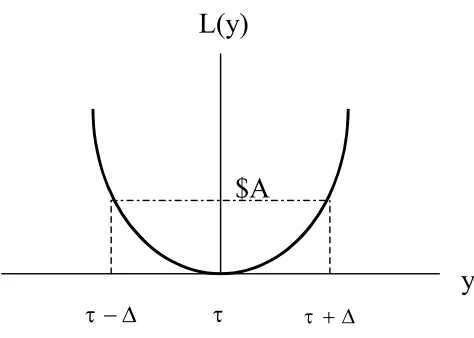
the deviation of its quality characteristic (denoted by Y) from a target value (denoted
τ +∆
τ
τ
−
∆
$A
y
L(y)
Figure 2-1: A Symmetric Loss Function
different from what we refer to asfraction defective, which implies that all products that
fall within specification limits (denoted byτ ±∆) are equally good (nondefective), while
those outside the specification limits are bad (defective). However, in reality, only the
product whose response is exactly on target yields the best performance. As the product’s
response deviates from the target the quality becomes progressively worse.
Figure 2-1 displays a symmetric continuous loss function. It presents a relationship
between the quality loss L(Y) and the amount of deviation from the target. As shown in
the figure the quality loss is zero when the quality characteristic is exactly on the target
(Y = τ); the quality loss keeps increasing as the quality characteristic deviates in either
direction from the target. At each specification limit the quality loss is equal to Adollars.
Note that A is the total cost of repair or replacement of a product. Taguchi [14], [15]
derived the quadratic loss function, which we will discuss next, using the information
2.1.1
Taguchi’s Derivation of the Quadratic Loss Function
Consider a quality characteristic whose value is represented by Y; we assume that the
target value ofY isτ.Deviations ofY fromτin either direction are considered undesirable.
Let L(Y) denote a function representing the monetary value (in dollars) of the losses
incurred by an arbitrary customer of a unit produced where the quality characteristic is
Y. We refer toL(Y)as the loss function forY. To approximately determine the function,
we expand it in the Taylor series about the target value τ up to the quadratic term as:
L(Y)≈L(τ) +L0(τ)(Y −τ) + L
00(τ)
2! (Y −τ)
2 (2.1)
Clearly, as shown in figure 2-1, we have L(τ) = 0. Also, since the minimum value of
the function occurs at this point thefirst derivative of the function evaluated atτ is zero.
Thus, the first two terms of (2.1) vanish and it would reduce to:
L(Y) = L
00(τ)
2! (Y −τ)
2 (2.2)
or
L(Y) =k(Y −τ)2 (2.3)
where kis a constant called quality loss coefficient.
Equation (2.3) is the conventional form of the quadratic loss function. We then need
to determine the proper value of the constant k. It is clear that the loss isAdollars when
(exactly on each specification limit). By applying this fact to Eq. (2.3) we obtain:
k= A
∆2
2.1.2
Derivation of the Expected Loss Based on the Quadratic Loss
Function
Certainly, the quality characteristic Y varies from unit to unit, and from time to time. It
is practical to represent its variation by a probability distribution function. Suppose that
the probability density function of Y is f(y). By having the quality loss function L(Y)
and the probability density function f(y) the expected loss per unit can be written in a
general form as:
E[L(Y)] =
∞
Z
−∞
L(y)f(y)dy (2.4)
In the case of the quadratic loss function we can substituteL(y)from Eq. (2.3) directly
into Eq. (2.4). By doing so we get
E[L(Y)] =
∞
Z
−∞
k(y−τ)2f(y)dy
= k£σ2Y + (µY −τ)2¤ (2.5)
2.2
Moment Estimation Using Taylor Series Approximation
In this section we discuss a means to relate the probability distributions of random input
variables Xi, for i= 1,2, . . . , n, to the probability distribution of the response Y, where
Y = h(X1, X2, . . . , Xn). Moment is one of the statistical tools for describing the
proba-bility distribution of a random variable. Assume that the random input variables Xi, for
i = 1,2, . . . , n, have the joint probability density function f(X1, X2, . . . , Xn); we define
the rth moments of Y about its mean, forr ≥2, whereY =h(X
1, X2, . . . , Xn) as:
E[(y−µY)r] =µrY =
∞
Z
−∞
. . .
∞
Z
−∞
| {z }
n
[h(x1, x2, . . . , xn)−µY]r·f(x1, x2, . . . , xn)dx1. . . dxn
(2.6)
where µY is the mean ofY,which is itself defined as
µY =
∞
Z
−∞
. . .
∞
Z
−∞
| {z }
n
h(x1, x2, . . . , xn)·f(x1, x2, . . . , xn)dx1. . . dxn (2.7)
As seen from Eqs. (2.6) and (2.7) evaluating the moments ofY directly from the defi
ni-tion would be computani-tionally difficult, if not impossible. Tukey [17] provided generalized
nonlinear propagation of error formulas for approximating up to the fourth moment of a
function of random variables. In this section we present the results of Tukey’s work. See
Tukey [17] for detailed discussion.
γi,Γi,and Gi,where
γi = µ
3 i (σ2 i) 3 2
Γi =
µ4
i (σ2i)2
Gi =
µ5
i
(σ2i)52
In the above definitionsµ3i, µ4i,andµ5i represent the 3rd, 4th, and 5th moment,
respec-tively, of Xi around its mean. We can estimate the first four moments of Y around its
mean, where Y =h(X1, X2, . . . , Xn), by applying the following formulas. Note that the
formulas presented here were originally derived by Tukey [17] and later revised by Evans
[2] to make some notations look simpler.
µY ≈ h(µ1, µ2, . . . , µn) +1 2
X
ihiiσ
2
i + 1 6
X
ihiiiγiσ
3
i + 1 24
X
ihiiiiΓiσ
4
i
+1 4
X
i<jhiijjσ
2
iσ2j + 1 120
X
ihiiiiiGiσ
5
i + 1 12
X
i6=jhiiijjσ
3
iσ2j
+terms of order higher than or equal to σ6
σ2Y ≈ X
ih
2
iσ2i +
X
ihihiiγiσ
3
i + 1 3
X
ihihiiiΓiσ
4 i + 1 4 X ih 2
ii(Γi−1)σ4i
+X
i<j
¡
hihijj +h2ij+hiijhj
¢
σ2iσ2j + 1
12
X
ihihiiiiGiσ
5
i
+1 6
X
ihiihiii(Gi−γi)σ
5
i +
X
i6=j
µ
1
2hihiijj+ 1
2hiihijj+hijhiij
+1 3hiiijhi
φY ≈ X ih
3
iγiσ3i + 3 2
X
ih
2
ihii(Γi−1)σ4i + 6
X
i<jhihjhijσ
2
iσ2j
+1 2
X
ih
2
ihiii(Gi−γi)σ5i + 3 4
X
ihih
2
ii(Gi−2γi)σ5i
+3X
i6=j
µ
hih2ij+ 1 2h
2
ihijj+hiihijhj+hihiijhj
γiσ3iσ2j
+terms of order higher than or equal toσ6
ϕY ≈ X
ih
4
i (Γi−3)σ4i + 2
X
ih
3
ihii(Gi−4γi)σ5i + 12
X
i6=jh
2
ihjhijγiσ3iσ2j
+terms of order higher than or equal toσ6+ 3¡σ2Y¢2
where
• µY is the mean ofY.
• σ2Y is the variance ofY.
• φY is the third moment of Y about its mean.
• ϕY is the fourth moment ofY about its mean.
• hi= ∂∂xhi
¯ ¯ ¯
µ1,µ2,... ,µn
, hii= ∂
2h
∂x2
i
¯ ¯ ¯
µ1,µ2,... ,µn
, hij= ∂
2h
∂xi∂xj
¯ ¯ ¯
µ1,µ2,... ,µn
,etc.
• The summations are from 1 to n.
2.3
Nonlinear Programming Approach to the Parameter
Design Problem
The problem of determining the optimal set points for controllable parameters of a product
or process is referred to as the parameter design problem. The problem was originally
formulated and successfully implemented by Taguchi [13]. Most authors who explored
this area employed the statistical design of experiment as the primary tools for studying
the problems, for example, see Fowlkers [7], Montgomery [9], Phadke [11], and Taguchi
[13], even in the cases where the analytical forms of the transfer functions are available.
However, in the case where the analytical form of a functional relationship between the
input parameters and the output variable, i.e. the transfer function, is available, or at least
can be well approximated, there is another strategy presented by Fathi [3], [5] to tackle
the parameter design problem. He proposed constrained nonlinear programming models
for this problem in which the expected loss or the variance of the response is minimized.
We devote the rest of this section discussing this concept briefly.
LetX1, X2, . . . , Xn be IID random variables withE(Xi) =µi and V ar(Xi) =σ2i,for
i= 1,2, . . . , n,and a response of interest can be defined analytically asY =h(X1, X2, . . . , Xn).
Therefore, Y is also a random variable whose probability distribution function depends
on the form of the function h(X1, X2, . . . , Xn) and the probability distribution functions
of X1 through Xn.
The basic idea of the parameter design problem is to determine the nominal values
of the controllable parameters (µ1, µ2, . . . , µn)that minimize the expected loss associated
may also be present and they need to be incorporated into the problem. By assuming the
quadratic loss function, as discussed earlier, an appropriate mathematical model for the
parameter design problem can be stated as:
Minimize E[L(Y)] =k£σ2
Y + (µY −τ)2
¤
Subject to (µ1, µ2, . . . , µn)∈M
where (µ1, µ2, . . . , µn) ∈ M represents possible constraints pertaining to the technical
requirements, processing cost, etc. of a certain problem. Note that in the model the
values of µY and σ2Y depend on the variables µ1 through µn as stated in the previous
section.
In general, the form of µY orσ2Y as a function of µ1 through µn may be difficult or,
in some circumstances, may be impossible to obtain. Usually, we have to approximate
them as discussed earlier. There are several means to approximate these parameters, see
Evan [2] and Fathi [5]. Several authors, for example, Fathi [3], [5], Montgomery [10], and
Phadke [11], adopted the compact version of formulas presented in the previous section, by
neglecting the higher-order terms, to approximate these parameters. The compact version
of the formulas for approximating µY and σ2
Y are in the forms:
µY ≈ h(µ1, µ2, . . . , µn) (2.8)
σ2Y ≈ X
ih
2
iσ2i (2.9)
where hi = ∂∂xhi
¯ ¯ ¯
µ1,µ2,... ,µn
and the summation is from 1 ton.
optimal values of µ1 through µn that minimize the expected loss associated with the
quality characteristic of interest. While keeping other parameters of the input variables
fixed µY and σ2Y can be expressed as functions of µ1 through µn. We use the notation
µ to represent the vector (µ1, µ2, . . . , µn). Therefore, µY and σ2Y as the functions of µ1 through µncan be written asµY(µ) andσ2Y(µ), respectively. By applying (2.8) and (2.9) for approximating µY(µ) and σ2
Y(µ),the above model can be restated as:
Minimize E[L(Y)] =k£σ2Y(µ) + (µY(µ)−τ)2¤ Subject to µY(µ) =h(µ)
σ2
Y(µ) =
P
i
µ ∂h
∂xi
¯ ¯ ¯
µ1,µ2,... ,µn
¶2
σ2
i
(µ)∈M
(PDME)
The mathematical model above is simply a constrained nonlinear programming
prob-lem that can be solved using an appropriate algorithm.
Nevertheless, while assuming the quadratic loss function, there is another way to model
the parameter design problem as discussed by many authors, for example, see Fathi [5],
Montgomery [10], and Phadke [11]. They suggested minimizing the variance of the quality
characteristic directly, while keeping its mean on the target. This leads to the following
mathematical model:
Minimize σ2Y(µ) =Pi
µ ∂h
∂xi
¯ ¯ ¯
µ1,µ2,... ,µn
¶2
σ2i
Subject to h(µ) =τ (µ)∈M
At this point an unavoidable question may come up as what are the differences between
these two models. It can be shown that the optimal solution to the (PDME) problem would
yield µY which may be slightly different fromτ,see Box [1].This difference is referred to
as the aim-offfactor. In order to avoid the aim-offfactor we can use (PDMV). However,
the optimal solution to the problem would yield slightly higher value of the expected loss
than what results from (PDME). See Fathi [3] for the discussion about this issue in more
detail. Later in this thesis, we will employ (PDME) to the parameter design problem
Chapter 3
Quartic Loss Function
As stated earlier there are two functional forms that are commonly used to represent
a quality loss function. One form is the conventional step function that is based on
classifying the units as defective and non-defective, and the other form is the quadratic
loss function that is proposed by Taguchi [14]. Either of these two functional forms has
a specific functional profile, and as a result we do not have any degrees of freedom in
choosing a desired functional profile in either context. This thesis proposes a loss function
that not only allows some degrees of flexibility in this regard, but it also can be applied
in the case where a non-symmetric function is desirable.
In this chapter we introduce a quartic loss function resulting from expanding the Taylor
series up to its quartic term. We then examine the appropriate values of the quality loss
coefficients in both cases where the function is symmetric and non-symmetric. Finally, we
present two simple examples that illustrate how the quartic loss function can provide a
3.1
Derivation of the Quartic Loss Function
Consider a quality characteristic whose value is represented byY, and we assume that the
target value ofY isτ.Deviations ofY fromτin either direction are considered undesirable.
Let L(Y) denote a function representing the monetary value (in dollars) of the losses
incurred by an arbitrary customer of a unit produced where the quality characteristic is
Y. We refer toL(Y)as the loss function forY. To approximately determine this function
we expand it in the Taylor series about the target value τ up to the fourth term as:
L(Y)≈L(τ) + L
0(τ)
1! (Y −τ) + L00(τ)
2! (Y −τ)
2+L000(τ)
3! (Y −τ)
3+L0000(τ)
4! (Y −τ) 4
(3.1)
Clearly we have L(τ) = 0. Also, since the minimum value of the function is attained
at the target τ, the first derivative of the function at this point is zero. Therefore, the
first two terms of (3.1) vanish. The equation would then reduce to
L(Y) = L
00(τ)
2! (Y −τ)
2+L000(τ)
3! (Y −τ)
3+ L0000(τ)
4! (Y −τ) 4
or we can rewrite as
L(Y) =k2(Y −τ)2+k3(Y −τ)3+k4(Y −τ)4 (3.2)
where k2, k3, and k4 are constants that we call second, third, and fourth ordered quality
loss coefficient, respectively. For reasons that we explain later in this chapter, we also
Equation (3.2) is the proposed quartic loss function. Instead of having only the
quadratic term as in the case of the quadratic loss function, we obtain two more
higher-order terms that represent the non-symmetry and the flexibility of the functional profile.
We then need to determine the proper values of k2, k3,and k4 that would make the loss
function behave in the way that we desire.
3.2
The Quality Loss Coe
ffi
cients
In this section we propose a methodology to determine the coefficients k2, k3, and k4
based on either case where the loss function is symmetric and non-symmetric, separately.
We initially examine the coefficients of a non-symmetric loss function; a symmetric loss
function is the special case.
3.2.1
Non-Symmetric Loss Function
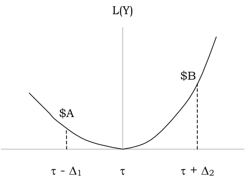
A non-symmetric loss function is shown in figure 3-1. The quality loss is zero when
the quality characteristic is exactly on the target τ; the quality loss keeps increasing
nonsymmetrically as the quality characteristic deviates in either direction from the target.
At the lower specification limit(τ−∆1)the quality loss is assumed to beAdollars, and at
the upper specification limit(τ+∆2)it is assumed to beBdollars. Note thatAandBare
all of the costs associated with the repair or replacement of a nonconforming unit at either
specification limit, respectively. We use the information fromfigure 3-1 to determine the
proper values of the constants k2, k3,and k4.
τ
$A
$B
τ
-
∆
1τ
+
∆
2L(Y)
Figure 3-1: A Non-Symmetric Loss Function (When ∆1 6=∆2).
• L(τ−∆1) =A
• L(τ+∆2) =B
• L00(Y)>0 − ∞< Y <∞
The last property holds because we assume that the loss function is convex everywhere
in(−∞,∞). We determine the values ofk2, k3,andk4 to satisfy these properties. At the
specification limits we have
L(τ −∆1) = A=k2∆21−k3∆31+k4∆41 (3.3)
Having solved Eqs. (3.3) and (3.4) fork2 and k3 in term of k4 we get
k2 =
Ã
1 1 +∆1
∆2
! µ
A
∆2 1
+∆1B
∆3 2
−(∆1∆2+∆21)k4
(3.5)
k3 =
Ã
1 1 +∆1
∆2
! µ
B
∆32 −
A
∆21∆2 + (∆
2 1
∆2 −
∆2)k4
(3.6)
It is clear that the coefficients can not be uniquely specified at this point. For any
value ofk4, however, the corresponding values ofk2 andk3 can be determined using these
equations. We now consider the property that imposes L00(Y) > 0, −∞ < Y < ∞. By
carrying out the second derivative of the quartic loss function (3.2) we have
L00(Y) = 2k2+ 6k3(Y −τ) + 12k4(Y −τ)2 (3.7)
Equation (3.7) can be rearranged in the form
L00(Y) = (12k4)Y2+ (6k3−24τk4)Y + (2k2−6τk3+ 12τ2k4) (3.8)
which is in the quadratic form
g(y) =ay2+by+c (3.9)
Observation In order for g(y) in Eq. (3.9) to be greater than zero for all values of y,
two conditions below need to be satisfied:
2. b2 <4ac
Proof. Equation (3.9) is in a parabolic form. To ensure thatg(y)is greater than zero,
it is required that two conditions below are true:
1. The function is convex, which implies that the function has a minimum point.
2. The minimum point of the function lies above zero.
For condition 1 to be true we need g00(y) > 0, for all −∞ < y < ∞. This condition
yieldsa >0.
For condition 2 to be true we need g(y)>0, where y is the global minimizer of g(y).
This condition yields b2<4ac.
Therefore, in order forL00(Y)to be greater than zero, we need to satisfy the following
conditions:
1. 12k4 >0
2. (6k3−24τk4)2<4(12k4)(2k2−6τk3+ 12τ2k4)
Which can be written as:
k4 > 0 (3.10)
k23 < 8
3k2k4 (3.11)
Substituting for k2 and k3 from Eqs. (3.5) and (3.6), respectively, we obtain the
1. k4 >0and
2. k4 is a value selected from the solutions to the following inequality:
·
(∆21−∆2 2)
2
∆2 2
+83³∆1∆22+2∆21∆2+∆31
∆2
´¸
k42+h³2∆B4 2 −
2A
∆2 1∆22
´ ¡
∆21−∆22¢
−83
³A(∆
1+∆2)
∆2
1∆2 +
∆1B(∆1+∆2)
∆4 2
´i
k4+
h B2 ∆6 2 − 2AB ∆2 1∆42
+ ∆A42 1∆22
i
<0
(3.12)
Any value of k4 that satisfies these inequalities leads to L00(Y) > 0. This typically
leads to a range of allowable value for k4, and we can select the values of k4 within this
range. The corresponding values of k2 and k3 are then determined using Eqs. (3.5) and
(3.6), respectively. The shape of the loss function depends on k4, which we previously
mentioned as the shape parameter, that we select from the allowable range, and we show
several examples illustrating the effect ofk4 on the functional profile later in this chapter.
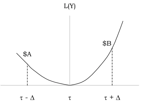
Now, let’s assume further that∆1 =∆2 =∆;in other words, the distances from the
targetτ to the lower specification limit(τ−∆)and to the upper specification limit(τ+∆)
are the same. At the lower specification limit(τ−∆1)the quality loss is assumed to beA
dollars, and at the upper specification limit (τ +∆2) it is assumed to beB dollars. This
is a special case of what we derived above. Figure 3-2 depicts this situation.
In this situation Eqs. (3.5) and (3.6) reduce to
k2 =
A+B
2∆2 −∆ 2k
4 (3.13)
k3 =
B−A
2∆3 (3.14)
de-τ
$A
$B
τ
-
∆
τ
+
∆
L(Y)
Figure 3-2: A Non-Symmetric Loss Function (When∆1=∆2 =∆)
termined in Eq. (3.14). The other two coefficients k2 and k4 can not be uniquely
speci-fied at this point. As before we need to include the property that requires L00(Y) > 0,
−∞< Y <∞. In this case, we havek4 >0 and (3.12) reduces to:
(2∆4)k42−(A+B)k4+ 3 8
(B−A)2
2∆4 <0 (3.15)
Note that (3.15) is the special form of (3.12), when ∆1 = ∆2 = ∆. After we select a
desired value of k4 we then use Eq. (3.13) to evaluate the corresponding value of k2.
3.2.2
Symmetric Loss Function
A symmetric loss function is the special case of what we presented in section 3.2.1, where
at each specification limit the quality loss is the same (i.e., A dollars). We use the same
procedure to evaluate the possible values of the coefficientsk2, k3,and k4.
The relationships would then be:
k2 =
A+A
2∆2 −∆ 2k
4 =
A
∆2 −∆
2k
4 (3.16)
k3 =
A−A
2∆3 = 0 (3.17)
The task would reduce to evaluating the feasible values of k4 and then substitute a
desired value of k4 into Eq. (3.16) to obtain k2. By using the same derivation as in the
previous section, the feasible range of k4 is:
1. k4 >0and
2. k4 is a value selected from the solutions to the following inequality:
(2∆4)k42−(2A)k4<0 (3.18)
It follows that 0< k4< ∆A4.
3.3
Examples
In this section we present two simple examples that illustrate how the quartic loss function
can provide a family of loss functions. The first example demonstrates the symmetric loss
function and the second one does the non-symmetric loss function with ∆1=∆2 =∆.
Example 3.1 We assume that the target value for a quality characteristic of interest in
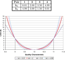
Table 3.1: The Chosen Values of k4 and Their Associated Values of k2 (Symmetric Loss Function)
Pair 1 2 3 4
k4 0.01 2.00 3.50 4.99
k2 4.99 3.00 1.50 0.01
0 1 2 3 4 5 6 7 8 9 10 11 12 13 14 15
8.5 9 9.5 10 10.5 11 11.5
Quality Characteristic
Loss ($)
k4 = 0.01 k4 = 2 k4 = 3.5 k4 = 4.99
Figure 3-3: A Family of Symmetric Loss Functions Corresponding to the Chosen Values of k4
Thus, this is the case where the loss function is symmetric with A = $5. We know
immediately from Eq (3.17) that k3 is zero. We then need to evaluate the feasible
range fork4 and then k2 can be solved by using Eq. (3.16). By using the procedure
provided in the previous section, k4 ∈ (0,5). We present here four profiles of the
quartic loss function based on four values of k4 : 0.01, 2, 3.5, and 4.99. Table 3-1
summarizes the four values of k4 and their associated values ofk2.Note that when
k4 = 0, L(Y) reduces to a quadratic loss function; and as we increase the value of
k4 the form of L(Y) becomes closer to the form of the conventional step function
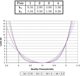
Table 3.2: The Chosen Values of k4 and Their Associated Values of k2 (Non-Symmetric Loss Function)
Pair 1 2 3 4
k4 0.16 2.00 4.00 5.30
k2 5.34 3.50 1.50 0.20
0 1 2 3 4 5 6 7 8 9 10 11 12 13 14 15
8.5 9 9.5 10 10.5 11 11.5
Quality Characteristic
Loss ($)
k4 = 0.16 k4 = 2 k4 = 4 k4 = 5.3
Figure 3-4: A Family of Non-Symmetric Loss Functions Corresponding to the Chosen Value ofk4
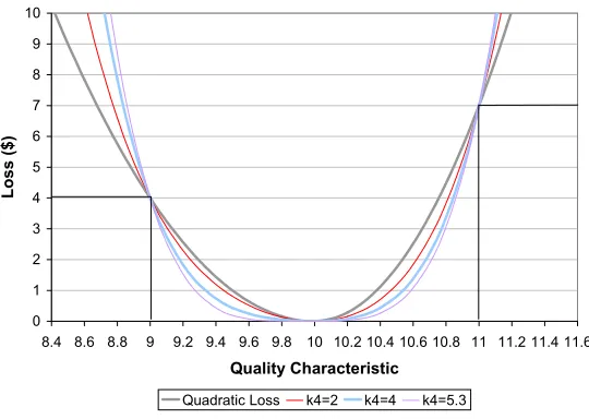
Example 3.2 This example is the embellishment of the previous example. Now let’s
as-sume that the cost for repairing or replacing an unacceptable product is not the same
at both specification limits (10±1), which implies the non-symmetric loss function
with∆1 =∆2=∆. Let’s assume that the repair cost at the lower specification limit
is A = $4, and at the upper specification limit it is B = $7. By using Eq. (3.14),
k3 = 1.5.Following the procedure in the previous section we havek4 ∈(0.158,5.342).
We present here four profiles of the quartic loss function based on four values ofk4 :
0.16, 2, 4, 5.3. Table 3-2 summarize the four values ofk4and their associated values
Conclusion Figures 3-3 and 3-4 depict various profiles of the symmetric and non-symmetric
loss functions, respectively, based onk4. Observe that within the specification
lim-its, as k4 decreases, at the same value of a quality characteristic the quality loss
increases. In other words, as k4 decreases the function would get steeper. At a large
value ofk4the loss function gets close to a step function within the specification
lim-its. At a small value ofk4the function becomes close to a quadratic loss function. A
decision maker can choose an appropriate value ofk4 in order to have a loss function
that represents a situation at hand. This process of choosing the appropriate value
Chapter 4
Expected Loss Based on the
Quartic Loss Function
In this chapter we develop expected loss formulas for a quartic loss function and present
two simple examples that illustrate the differences among expected losses attained by
assuming the quadratic loss function, the quartic loss function, and the step function.
4.1
Derivation of the Expected Loss Formulas
Because a quality characteristic Y varies from unit to unit and from time to time, it is
practical to represent its variation by a probability distribution function. Let f(y) be
the probability density function of Y. By having the quality loss function L(Y) and the
form as
E[L(Y)] =
∞
Z
−∞
L(y)f(y)dy (4.1)
The quartic loss function is in the form:
L(y) =k2(y−τ)2+k3(y−τ)3+k4(y−τ)4
Therefore, the expected loss can be derived as:
E[L(Y)] =
∞
Z
−∞
{k2(y−τ)2+k3(y−τ)3+k4(y−τ)4}f(y)dy
= k2
∞
Z
−∞
[(y−µY) + (µY −τ)]2f(y)dy+k3
∞
Z
−∞
[(y−µY) + (µY −τ)]3f(y)dy
+k4
∞
Z
−∞
[(y−µY) + (µY −τ)]4f(y)dy
= k2
£
σ2Y + (µY −τ)2¤+k3
£
φY + 3σ2Y(µY −τ) + (µY −τ)3¤
+k4
£
ϕY + 4φY(µY −τ) + 6σ2Y(µY −τ)2+ (µY −τ)4¤ (4.2)
where
• µY is the mean ofY.
• σ2Y is the variance ofY.
• ϕY is the fourth moment ofY about its mean.
For the symmetric case, k3 = 0, as shown earlier in the thesis. Thus, (4.2) would
reduce to
E[L(Y)] = k2
£
σ2Y + (µY −τ)2¤+k4
£
ϕY + 4φY(µY −τ) + 6σ2Y(µY −τ)2 (4.3)
+(µY −τ)4¤
4.2
Examples
In this section we present two simple examples that illustrate the differences of the expected
loss per unit when we base our analysis on a quadratic loss function, a quartic loss function,
and a step function.
Example 4.1 Let Y be a quality characteristic of interest of a product. Assume again
that the desired value of Y is τ = 10 and its specification limits are 10±1, or
∆= 1. The cost for repairing or replacing an unacceptable product is $5 at either
specification limit, or A= 5.
Figure 4-1 depicts a quadratic loss function, a family of quartic loss functions, and a
step function that represent the given situation. Note that the quartic loss functions
are those between the quadratic loss function and the step function. The quartic
loss coefficients applied here are the same as those we used in example 3.1.
Suppose that Y is normally distributed with mean µY = 10, and variance σ2Y. We
0 1 2 3 4 5 6 7 8 9 10
8.4 8.6 8.8 9 9.2 9.4 9.6 9.8 10 10.2 10.4 10.6 10.8 11 11.2 11.4 11.6
Quality Characteristic
Loss ($)
Quadratic Loss k4=2 k4=3.5 k4=4.8
Figure 4-1: Symmetric Loss Functions representing the Scenario
loss function and Eq. (4.3) to determine the value based on the quartic loss function.
Since Y is normally distributed φY = 0, and ϕY = 3σ4Y. Note that ΓY = 3 for a
normal distribution.We apply the following relationship to determine the expected
loss per unit based on the step function:
E[L(Y)] =A×(1−Pr{τ−∆6Y 6τ +∆})
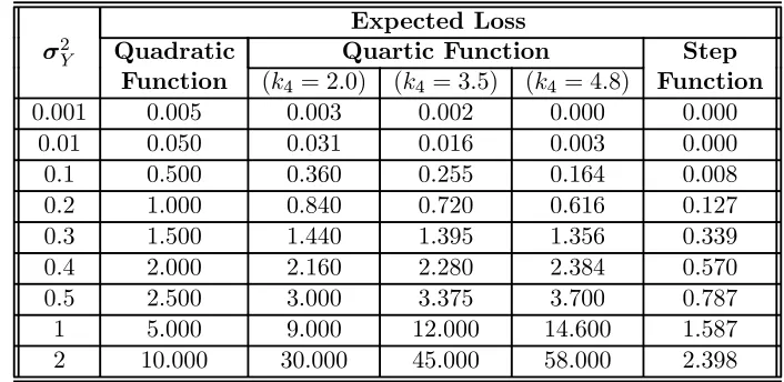
The results of the calculation for different values ofσ2Y are shown in table 4.1. Each
row of the table corresponds to a different value ofσ2Y, and we present three different
values of the shape parameter k4 for the quartic loss function.
We make the following observations from table 4.1:
• At smaller value of σ2Y the expected loss per unit based on the quartic loss
Table 4.1: Expected Losses at Some Values of Variance of Y (Symmetric Case with Mean = 10)
Expected Loss
σ2Y Quadratic Quartic Function Step
Function (k4 = 2.0) (k4 = 3.5) (k4 = 4.8) Function
0.001 0.005 0.003 0.002 0.000 0.000
0.01 0.050 0.031 0.016 0.003 0.000
0.1 0.500 0.360 0.255 0.164 0.008
0.2 1.000 0.840 0.720 0.616 0.127
0.3 1.500 1.440 1.395 1.356 0.339
0.4 2.000 2.160 2.280 2.384 0.570
0.5 2.500 3.000 3.375 3.700 0.787
1 5.000 9.000 12.000 14.600 1.587
2 10.000 30.000 45.000 58.000 2.398
hand, when the variance of Y is larger the expected loss per unit based on the
quartic loss functions is greater than that based on the quadratic loss function.
This incident can be best explained byfigure 4-1. Within the specification
lim-its less penalty would be charged to any products whose quality characteristics
deviate from the target when we apply the quartic loss functions. However,
beyond the limits, more penalty would be charged. When σ2Y is small as
com-pared with ∆most units fall within the specification limits and; therefore, less
penalty is charged to the units whose quality characteristics deviate from the
target. As σ2Y gets larger there would be more units whose quality
character-istics fall outside the limits, and these units are in fact charged with severe
penalty. This penalty is much more than that inside the specification limits
and tend to predominate on the value of the expected loss.
• For the quartic loss functions, at small value of σ2
Y the expected loss per unit
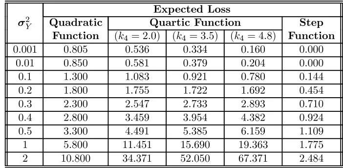
Table 4.2: Expected Losses at Some Values of Variance of Y (Symmetric Case with Mean = 9.6)
Expected Loss
σ2Y Quadratic Quartic Function Step
Function (k4 = 2.0) (k4 = 3.5) (k4 = 4.8) Function
0.001 0.805 0.536 0.334 0.160 0.000
0.01 0.850 0.581 0.379 0.204 0.000
0.1 1.300 1.083 0.921 0.780 0.144
0.2 1.800 1.755 1.722 1.692 0.454
0.3 2.300 2.547 2.733 2.893 0.710
0.4 2.800 3.459 3.954 4.382 0.924
0.5 3.300 4.491 5.385 6.159 1.109
1 5.800 11.451 15.690 19.363 1.775
2 10.800 34.371 52.050 67.371 2.484
expected loss per unit increases as k4 increases. The same argument as that in
the previous observation can be used to explain this incident.
• The expected loss per unit based on the step function is the smallest no matter
how large σ2Y is since no penalty is charged to any unit whose quality
charac-teristic falls within the specification limits. Moreover, a constant rate of $5 is
charged on the products whose quality characteristics fall outside the limits.
Now, assume that the mean of Y equals to 9.6, which deviates slightly from
the target while we keep the other assumptions the same. Table 4.2 summarizes the
expected loss per unit based on each kind of loss function as we vary σ2Y.The same
conclusion can be inferred. However, since the mean of Y is not exactly on target,
the overall expected loss per unit for this situation is higher. Furthermore, it is
obvious that the percentage difference between the expected loss per unit resulting
from this situation and that resulting from the previous one is large at the small
0 1 2 3 4 5 6 7 8 9 10
8.4 8.6 8.8 9 9.2 9.4 9.6 9.8 10 10.2 10.4 10.6 10.8 11 11.2 11.4 11.6
Quality Characteristic
Loss ($)
Quadratic Loss k4=2 k4=4 k4=5.3
Figure 4-2: Non-Symmetric Loss Functions representing the Scenario
Example 4.2 We consider the case as described in the previous example, except that we
now assume that the cost for repairing or replacing an unacceptable product is $4
at the lower limit, or A= 4and $7 at the upper limit, orB= 7.
Figure 4-2 depicts a quadratic loss function, a family of quartic loss functions, and
a step function that represent the given situation. Note that the quartic loss
func-tions are those between the quadratic loss function and the step function within the
specification limits. The quartic loss coefficients applied here are the same as those
we used in example 3.2. We evaluated the quadratic loss coefficients using:
kL =
A
∆2
kU =
B
∆2
Table 4.3: Expected Losses at Some Values of Variance of Y (Non-Symmetric Case with Mean = 10)
Expected Loss
σ2Y Quadratic Quartic Function Step
Function (k4 = 2.0) (k4 = 4.0) (k4 = 5.3) Function
0.001 0.0055 0.004 0.002 0.000 0.000
0.01 0.055 0.036 0.016 0.004 0.000
0.1 0.550 0.410 0.270 0.179 0.009
0.2 1.100 0.940 0.780 0.676 0.139
0.3 1.650 1.590 1.530 1.491 0.373
0.4 2.200 2.360 2.520 2.624 0.626
0.5 2.750 3.250 3.750 4.075 0.865
1 5.500 9.500 13.500 16.100 1.745
2 11.000 31.000 51.000 64.000 2.637
In effect we assume that we have two different quadratic loss functions, one for each
side of the target value.
Suppose that Y is normally distributed with mean µY = 10, and variance σ2Y. We
carry out the analysis for different values ofσ2Y as shown in thefirst column of table
4.3. Table 4.3 summarizes the expected loss per unit based on each kind of loss
function as we varyσ2Y.The same conclusion as that of the previous example can be
inferred. Notice that the overall expected loss per unit is slightly higher than what
resulted from the previous example since more penalty is charged to any products
whose quality characteristics deviate to the right side of the target.
It may be of interested to know what would happen if the mean ofY deviates slightly
to the left side of the target. Now, assume that the mean of Y equals 9.99. Table
4.4 summarizes the expected loss per unit based on each kind of loss function as we
varyσ2
Y.Notice that the overall values of the expected loss per unit is less than the
Table 4.4: Expected Losses at Some Values of Variance of Y (Non-Symmetric Case with Mean = 9.99)
Expected Loss
σ2Y Quadratic Quartic Function Step
Function (k4 = 2.0) (k4 = 4.0) (k4 = 5.3) Function
0.001 0.0056 0.0038 0.0016 0.0002 0.0000
0.01 0.0543 0.0355 0.0159 0.0032 0.0000
0.1 0.5468 0.4060 0.2659 0.1748 0.0084
0.2 1.0952 0.9316 0.7716 0.6677 0.1374
0.3 1.6440 1.5772 1.5174 1.4785 0.3695
0.4 2.1930 2.3428 2.5031 2.6073 0.6210
0.5 2.7421 3.2285 3.7289 4.0541 0.8591
1 5.4886 9.4566 13.4576 16.0582 1.7381
2 10.9836 30.9128 50.9150 63.9164 2.6307
shifting the mean ofY slightly to the left side of the target, where the average cost
at the lower specification limit is less than that at the upper limit, can help reduce
the expected loss per unit. However, if we shift the mean of Y further to the left,
the overall expected loss per unit will increase.
For example, let’s assume that the mean of Y is now equal to 9.6. Table 4.5
sum-marizes the expected loss per unit based on each kind of loss function as we vary
σ2Y. This time, as we mentioned, the overall expected loss per unit increases, and
shifting the mean ofY too far from the target can not help reduce the expected loss
Table 4.5: Expected Losses at Some Values of Variance of Y (Non-Symmetric Case with Mean = 9.6)
Expected Loss
σ2Y Quadratic Quartic Function Step
Function (k4 = 2.0) (k4 = 4.0) (k4 = 5.3) Function
0.001 0.6440 0.519 0.250 0.075 0.000
0.01 0.6800 0.552 0.283 0.108 0.000
0.1 1.1203 0.937 0.720 0.579 0.116
0.2 1.6404 1.479 1.434 1.105 0.366
0.3 2.1610 2.141 2.388 2.549 0.584
0.4 2.6828 2.923 3.582 4.011 0.780
0.5 3.2059 3.825 5.016 5.791 0.959
1 5.8391 10.135 15.786 19.460 1.662
Chapter 5
Mathematical Model for the
Parameter Design Problem and a
Case Study
In this chapter we present a mathematical model for the parameter design problem
based on the quartic loss function assumption. Throughout the chapter we assume
that the functional relationship of input parameters and a quality characteristic, i.e.
Y = h(X1, X2, . . . , Xn), is well defined in a closed form or at lease could be well
ap-proximated. We then provide a case study for either case where the loss function is
symmetric and non-symmetric. For the case of symmetric loss function we also compare
5.1
The Model
The parameter design problem is the problem of determining optimal set points for design
variablesX1throughXnof a product or a process. The basic idea of the parameter design
problem is to identify nominal values of the design variables µ1 through µnthat minimize
the expected loss associated with a quality characteristic Y.
LetX= (X1, X2, . . . , Xn)be a vector of design variables (components) for a product
or a process, and letY =h(X1, X2, . . . , Xn)represents a quality characteristic of interest.
We consider X1 through Xn to be random variables with respective nominal values µ1
through µn. Thus, Y = h(X1, X2, . . . , Xn) is also a random variable whose probability
density function and its associated parameters depend on the form of the transfer function
and the probability density functions of X1 through Xn,as well as on their corresponding
parameters. As discussed in the previous chapter the expected loss ofY depends on some
of its lower moments which, in fact, depend on the parameters ofX1throughXn.However,
for the parameter design problem we consider µ1 through µn as controllable parameters
and the other parameters are fixed.
We therefore define the parameter design problem to be the problem of determining
an optimal set of values for µ1 through µn that minimizes the expected loss associated
with the quality characteristicY. In most applications some constraints pertaining to the
loss function the problem can be expressed mathematically as the following model:
Minimize E[L(Y)] =k2
£
σ2Y + (µY −τ)2¤+k3
£
φY + 3σ2Y(µY −τ) + (µY −τ)3¤
+k4£ϕY + 4φY(µY −τ) + 6σY2(µY −τ)2+ (µY −τ)4
¤
Subject to (µ1, µ2, . . . , µn)∈M
where (µ1, µ2, . . . , µn) ∈ M represents possible constraints pertaining to the technical
requirements, processing cost, etc. of a certain problem.
Obviously the values of these parameters,µY,σ2
Y,φY,and ϕY,depend on the design
parameters µ1 through µn.However, these functional relationships may be difficult, or in
some cases even impossible to obtain in closed forms, and we usually have to approximate
them. There are several means to approximate these parameters (see Evan [2]). In this
thesis we adopt the approximation method presented by Tukey [17] as we discussed in
Chapter 2, and we assume that X1, X2, . . . , Xn are IID random variables with known
parameters σ2
i,γi,andΓi.
The formulas for estimating up to the fourth moment of the quality characteristicY
are presented below. Note that we include here all terms up to the terms of order σ4.
The original work by Tukey [17] and the revised version by Evans [2] contained up to
the terms of order σ5 in their formulas. Including the terms of order σ5 would require
exhausting efforts; however, they can barely improve the accuracies of the approximation
to include them in our analysis.
µY ≈ h(µ1, µ2, . . . , µn) +1 2
X
ihiiσ
2
i + 1 6
X
ihiiiγiσ
3
i
+ 1
24
X
ihiiiiΓiσ
4
i + 1 4
X
i<jhiijjσ
2
iσ2j (5.1)
σ2Y ≈ X
ih
2
iσ2i +
X
ihihiiγiσ
3
i + 1 3
X
ihihiiiΓiσ
4 i +1 4 X ih 2
ii(Γi−1)σ4i +
X
i<j
¡
hihijj+h2ij+hiijhj
¢
σ2iσ2j (5.2)
φY ≈ X
ih
3
iγiσ3i + 3 2
X
ih
2
ihii(Γi−1)σ4i + 6
X
i<jhihjhijσ
2
iσ2j (5.3)
ϕY ≈ X
ih
4
i (Γi−3)σ4i + 3
¡
σ2Y¢2 (5.4)
where
• hi= ∂∂xh
i
¯ ¯ ¯µ
1,µ2,... ,µn
, hii= ∂
2h
∂x2
i
¯ ¯ ¯
µ1,µ2,... ,µn
, hij= ∂
2h
∂xi∂xj
¯ ¯ ¯µ
1,µ2,... ,µn
,etc.
• The summations are from 1 to n.
By applying these formulas the values of µY, σ2Y, φY, and ϕY can be expressed as
Minimize k2
h
σ2Y(µ) +{µY(µ)−τ}2i+k3
£
φY(µ) + 3σ2Y(µ){µY(µ)−τ} +{µY(µ)−τ}3
i
+k4[ϕY(µ) + 4φY(µ){µY(µ)−τ} + 6σ2
Y(µ){µY(µ)−τ}2+{µY(µ)−τ}4
i
Subject to µY(µ) =h(µ) +21Pihiiσ2i + 16
P
ihiiiγiσ3i +241
P
ihiiiiΓiσ4i
+14Pi<jhiijjσ2iσ2j
σ2Y(µ) =Pih2iσ2i +Pihihiiγiσ3i +13
P
ihihiiiΓiσ4i
+14Pih2ii(Γi−1)σ4i +
P
i<j
³
hihijj +h2ij+hiijhj
´
σ2iσ2j
φY(µ) =Pih3iγiσ3i +23Pih2ihii(Γi−1)σ4i + 6
P
i<jhihjhijσ2iσ2j
ϕY(µ) =Pihi4(Γi−3)σ4i + 3
¡
σ2Y(µ)¢2
(µ)∈M
(PDM)
where, as in the previous chapter
• hi= ∂∂xhi
¯ ¯ ¯
µ1,µ2,... ,µn
, hii= ∂
2h
∂x2
i
¯ ¯ ¯
µ1,µ2,... ,µn
, hij= ∂
2h
∂xi∂xj
¯ ¯ ¯
µ1,µ2,... ,µn
,etc.
• All summations are from 1 to n.
The model is a nonlinear constrained optimization problem which we can solve by a
nonlinear programming software package, such as LINGO or the Excel Solver.
5.2
A Case Study
of a quartic loss function, which depends on the shape parameter k4, has an effect on the
optimal solutions. For the case of a symmetric function we also compare the results with
what we would obtain by using a quadratic loss assumption.
5.2.1
The Problem Statement
We consider a coil spring loaded in tension or compression. We define the following
notations and data for the problem formulation:
Shear modulus: G= 1.15×10⁷ (lb/in2)
Weight density of a spring material: V = 0.285(lb/in3)
Gravitational constant: g= 386(in/sec2)
Mass density of the spring material: ρ= Vg = 7.38342×10⁻⁴ (lb-sec2/in4)
Deflection along the axis of the spring when it is loaded: δ (in)
Shear stress: S (lb/in2)
Frequency of surge waves: ω (Hz)
Applied load: P (lbs)
The deflection (δ) is the performance characteristic of the coil spring with a desired
target of 0.5 inches when a load of P = 1000 lbs is applied. The shear stress (S) and
the surge waves (ω)are the technical requirements whose values should be within certain
limits for a proper function of the coil spring. These issues will be discussed later in this
subsection.
Wire diameter: d(in.)
Coil diameter: D(in.)
Number of active coils: N
The relevant technical relationships are given below:
1. Load deflection equation:
P =
µ
d4G 8D3N
δ (5.5)
2. Shear stress equation:
S= 8P D
πd3
µ
4D−d 4(D−d) +
0.615d D
(5.6)
3. Frequency of surge waves equation:
ω= d
2πD2N
s
G
2ρ (5.7)
We consider d, D, and N to be pairwise independent normal random variables with
respective means µd,µD,and µN; respective variancesσ2d,σ2D,and σ2N. We assume that
σd= 0.006,σD= 0.025,σN = 0.2,and since all random variables are normally distributed
we have γd=γD=γN = 0,and Γd=ΓD=ΓN = 3.
In the context of this problemµd,µD,andµN are the decision variables, and we want to
problem, we are now ready to formulate the preliminary relationships for the parameter
design problem in term of µd,µD,andµN.
The deflection of the spring under an applied load of 1000 lbs (the performance
char-acteristic of the problem) can be formulated by using Eq. (5.5):
δ= D
3N
1437.5d4 (5.8)
The maximum allowable shear stress in this problem was given to be 80,000 lb/in2.
This requirement can be formulated by using Eq. (5.6):
636.62D(4D−d) d3(D−d) +
1566.084
d2 ≤80,000 (5.9)
To avoid serious resonance in dynamic applications the frequency of surge waves must
be at least 100 Hz. This requirement can be formulated by using Eq. (5.7):
14045.1d
D2N ≥100 (5.10)
The outer diameter of the coil spring is required to be no bigger than 2.5 inches. This
requirement can be formulated as:
Finally, we have the following explicit bounds on the decision variables.
0.2 ≤ µd≤0.8
0.9 ≤ µD≤2 (5.12)
2 ≤ µN ≤25
5.2.2
Symmetric Loss Function
As discussed in section 5.2.1 the desired target of deflection when a load of 1000 lbs is
applied is τ = 0.5 inches. We assume that the specification limits are 0.5±0.04; and the
losses at each limit is $5. In order to solve the parameter design problem wefirst need to
determine the proper value of the coefficients k2, k3, and k4. In this case k3 is zero since
the function is symmetric. Only k2 andk4 are left to be evaluated.
By applying the procedure discussed in chapter 3, k4 ∈ (0,1953125). Recall that for
the case of symmetric loss function, k4 needs to satisfy two conditions; i) k4 >0, and ii)
k4 must satisfy the inequality (3.18). We solvefive parameter design problems here with
five values of the shape parameter; k4 =0, 100, 100000, 1000000, and 1953124. By Using
Eq. (3.16) we can determine their associated k2= 3125, 3124.84, 2965, 1525, and 0.0016,
respectively. When k4 = 0 we have the quadratic loss function. Figure 5-1 depicts the
various profiles of the loss functions when we vary the values ofk4.Note that the profiles
of the functions whenk4 = 0,k4= 100, and k4 = 100000 are almost identical.
We are now ready to formulate a parameter design model. We demonstrate here only
0 1 2 3 4 5 6 7
0.45 0.46 0.47 0.48 0.49 0.5 0.51 0.52 0.53 0.54 0.55
Deflection (inches)
Loss ($)
k=0 k4 = 100 k4 = 100000 k4 = 1000000 k4 = 1953124
Figure 5-1: Effects ofk4 on the Symmetric Loss Functions
similar way. By applying the proposed model (PDM), the model for this specific problem
Min 3124.84hσ2δ(µ) +{µδ(µ)−0.5}2i+ 100 [ϕδ(µ) + 4φδ(µ){µδ(µ)−0.5} +6σ2δ(µ){µδ(µ)−0.5}2+{µδ(µ)−0.5}4i
Subject to µδ(µ) = 14371.5nhµ3DµN
µ4
d
i
+h³3µDµN
µ4
d
´
(0.025)2+³10µ3DµN
µ6
d
´
(0.006)2i
+h³105µ3DµN
µ8
d
´
(0.006)4i+h³30µDµN
µ6
d
´
(0.025)2(0.006)2io
σ2δ(µ) = 14371.52
½·³3µ2
DµN
µ4
d
´2
(0.025)2+³−4µ3DµN
µ5
d
´2
(0.006)2+³µ3D
µ4
d
´
(0.2)2i+h³3µ2DµN
µ4
d
´ ³6µ
N
µ4
d
´
(0.025)4+³−4µ3DµN
µ5
d
´ ³
−120µ3DµN
µ7
d
´
(0.006)4i+1 2
·³6µ
DµN
µ4
d
´2
(0.025)4+³20µ3DµN
µ6
d
´2
(0.006)4
¸
·µ³3µ2
DµN
µ4
d
´ ³60µ2
DµN
µ6
d
´
+³−12µ2DµN
µ5
d
´2
+³−24µDµN
µ5
d
´ ³
−4µ3DµN
µ5
d
´
(0.025)2(0.006)2+µ³3µ2D
µ4
d
´2
+³6µD
µ4
d
´ ³µ3
D
µ4
d
´
(0.025)2(0.2)2
µ³µ3
D
µ4
d
´ ³20µ3
D
µ6
d
´
+³−4µ3D
µ5
d
´2
(0.2)2(0.006)2
¸¾
φδ(µ) = 14371.53
½
3·³3µ2DµN
µ4
d
´2³6µ
DµN
µ4
d
´
(0.025)4+³−4µ3DµN
µ5
d
´2³20µ3
DµN
µ6
d
´
(0.006)4i+ 6h³3µ2DµN
µ4
d
´ ³
−4µ3DµN
µ5
d
´ ³
−12µ2DµN
µ5
d
´
(0.025)2(0.006)2
+³3µ2DµN
µ4
d
´ ³µ3
D
µ4
d
´ ³3µ2
D
µ4
d
´
(0.025)2(0.2)2+³µ3D
µ4
d
´ ³
−4µ3DµN
µ5
d
´ ³ −4µ3D
µ5
d
´
(0.2)2(0.006)2io
ϕδ(µ) = 3¡σ2
δ(µ) ¢2
636.62µD(4µD−µd)
µ3
d(µD−µd) +
1566.084
µ2
d ≤
80,000
14045.1µd
µ2
DµN ≥100
µD+µd≤2.5
0.2≤µd≤0.8, 0.9≤µD≤2, 2≤µN ≤25
We solved this model and the other four models using the software package LINGO
on a celeron 700 MHz personal computer. The results are displayed in Table 5-1. Notice
Table 5.1: Summary of the Results (Symmetric Loss Function)
Assumption µd µD µN E[L(y)] µδ σδ
k4= 0(Quadratic Loss Function) 0.6780 1.8220 25 $2.35 0.4984 0.0274
k4 = 100 0.6780 1.8220 25 $2.35 0.4984 0.0274
k4 = 100000 0.6781 1.8219 25 $2.40 0.4982 0.0274
k4= 1000000 0.6783 1.8217 25 $2.81 0.4974 0.0273
k4= 1953124 0.6784 1.8216 25 $3.25 0.4970 0.0273
this incident at thefirst glance; however, with careful analysis, we found that the optimal
solutions yielded σδ around 0.027, which is relatively large comparing with ∆ = 0.04.
As the result, many springs whose quality characteristics fell outside the specification
limits were charged with severe penalty. This penalty is much more than that inside the
specification limits and tend to predominate on the value of the expected loss. Besides, as
we increase k4 the penalty charged on a nonconforming unit noticeably increases. Thus,
these are the reasons why the optimal value of expected loss increases as we increase k4.
Now, consider the case when we assume that the specification limits are wider, and
observe the result. Assume that the specification limits are now 0.5±0.1 while we keep
every parameter the same as before. By applying the procedure discussed in chapter 3
k4 ∈(0,50000). We solvefive parameter design problems here withfive values of the shape
parameter; k4=0, 100, 10000, 30000, and 49990. By Using Eq. (3.16), we can determine
their associated k2 = 500, 499, 400, 200, and 0.1, respectively. Figure 5-2 depicts the
various profiles of the loss functions when we vary the values ofk4.Note that the profiles
of the functions whenk4 = 0and whenk4= 100are almost identical.
We solved this embellishment using the software package LINGO on a celeron 700 MHz
personal computer. The results of the parameter design problem based on this situation
0 1 2 3 4 5 6 7
0.35 0.4 0.45 0.5 0.55 0.6 0.65
Deflection (inches)
Loss ($)
k=0 k4 = 100 k4 = 10000 k4 = 30000 k4 = 49990
Figure 5-2: Effects ofk4 on the Symmetric Loss Functions (Embellishment)
Table 5.2: Summary of the Results (Symmetric Loss Function with Embellishment)
Assumption µd µD µN E[L(y)] µδ σδ
k4= 0(Quadratic Loss Function) 0.6780 1.8220 25 $0.38 0.4984 0.0274
k4 = 100 0.6780 1.8220 25 $0.38 0.4984 0.0274
k4 = 10000 0.6781 1.8219 25 $0.32 0.4983 0.0273
k4 = 30000 0.6782 1.8218 25 $0.20 0.4978 0.0273
k4 = 49990 0.6784 1.8216 25 $0.08 0.4970 0.0273
we widened the specification limits, while the optimal solutions yielded the sameσδ,most
of the produced springs would fall within the new limits. The penalty is not severe within
the specification limits and as we increase k4 the penalty is even less severe. Thus, these
are the reasons why the optimal value of expected loss decreases as we increasek4.
5.2.3
Non-Symmetric Loss Function
As discussed in section 5.2.1 the desired target of deflection when a load of 1000 lbs is
0 1 2 3 4 5 6 7 8 9 10 11 12 13 14 15
0.45 0.46 0.47 0.48 0.49 0.5 0.51 0.52 0.53 0.54 0.55
Deflection (inches)
Loss ($)
k4=24675 k4=1000000 k4=2319000
Figure 5-3: Effects of k4 on the Non-Symmetric Loss Functions.
order to solve the parameter design problem wefirst need to determine the proper values
of the quality loss coefficientsk2, k3,and k4.
By applying the procedure discussed in chapter 3 k4 ∈ (24673.83,2319076.17). Once
again recall that for the case of non-symmetric loss function with ∆1 = ∆2 = ∆, the
shape paremeterk4 needs to satisfy the two conditions stated in the inequality (3.15). We
solve three parameter design problems here with three values of the shape parameter;k4 =
24675, 1000000, and 2319000. By using Eq. (3.13) we can determine their associatedk2 =
3710.52, 2150, and 39.6, respectively. By Using Eq. (3.14) we can determinek3 = 15625.
Figure 5-3 depicts the various profiles of the quality loss function when we vary the values
of k4.
We are now ready to formulate a parameter design model. We exhibit only the model
with k2 = 3710.52 and k4 = 24675.The other models can be formulated in a similar way.