ABSTRACT
MURAD, NEHA. Quantitative Modeling and Optimal Control of Immunosuppressant Treatment Dynamics in Renal Transplant Recipients. (Under the direction of H.T. Banks.)
Individuals undergoing kidney transplants are put on a lifetime supply of immunosuppression
to prevent an allograft rejection. However suboptimal immunosuppressive therapy can put a
renal transplant recipient at a risk of infection. The key to a successful transplant is finding the optimal balance between over-suppression and under-suppression of the immune response, a task
which is difficult to achieve in renal transplant patients due to the narrow therapeutic index of
immunosuppressants. BK virus is a pathogen known to be a leading cause of kidney failure in renal transplant recipients. This pathogen has no antiviral therapy and can only be controlled by the
body’s immune response. This sole dependance on the immune system to curb BKV infections
makes optimization of the immunosuppression therapy an even more pertinent problem to solve. In this dissertation, we first examine uncertainty in clinical data from a kidney transplant recipient
infected with BK virus and investigate mathematical model and statistical model misspecification
in the context of least squares methodology. A difference-based method is directly applied to data to determine the correct statistical model that represents the uncertainty in data. We then carry
out an inverse problem with the corresponding iterative weighted least squares technique and use
the resulting modified residual plots to detect mathematical model discrepancy. This process is implemented using both clinical and simulated data. Our results demonstrate mathematical model
misspecification when both simpler and more complex models are assumed compared to data
dynamics. Our ultimate goal is to apply control theory to adaptively predict the optimal amount of immunosuppression in renal transplant recipients; however, we first need to formulate a biologically
realistic model. The process of quantitively modeling biological processes is iterative and often
leads to new insights with every iteration. We illustrate this iterative process of modeling for renal transplant recipients infected by BK virus. We analyze and improve on the current mathematical
model by modifying it to be more biologically realistic and amenable for designing an adaptive
treatment strategy. We use the improved model to design our feedback control loop applying Receding Horizon Control (RHC) methodology. Since data is not available for all model states
we use Non Linear Kalman Filtering (specifically Extended Kalman Filter (EKF)) to estimate the non-measurable states. Combining RHC and EKF we design an adaptive treatment plan which
© Copyright 2018 by Neha Murad
Quantitative Modeling and Optimal Control of Immunosuppressant Treatment Dynamics in Renal Transplant Recipients
by Neha Murad
A dissertation submitted to the Graduate Faculty of North Carolina State University
in partial fulfillment of the requirements for the Degree of
Doctor of Philosophy
Biomathematics
Raleigh, North Carolina
2018
APPROVED BY:
Alun Lloyd Justin Post
Hien Tran H.T. Banks
DEDICATION
The journey that has led me here, hasn’t always been easy. Over the years, I have come to believe
that impediments, while they may seem like annoyances and hindrances, are one’s biggest assets. If I have succeeded today it’s not in spite of my challenges, it is because of them.
This dissertation is dedicated to all the people who have stood by me through thick and thin.
BIOGRAPHY
Neha Murad was born on December 18th, 1988 in the city of joy, Kolkata, India. She was raised in
Kolkata and attended an all girls convent school, Our Lady Queen of the Missions. In 2007, she en-rolled in the Mathematics honors program at St. Xavier’s College, Kolkata. She graduated First Class
(a distinction secured by less than 1% candidates) and received her B.Sc in Mathematics honors degree in 2010. She went on to get an M. Sc. degree in Mathematics from Jadavpur University. It
was in Jadavpur University that she was first exposed to the scope of mathematical applications in
biology. After graduating with an M.Sc. in Mathematics in 2013, Neha left her hometown Kolkata for the first time to go to University of Iowa to pursue her Ph.D. in Applied Mathematics. While
exploring various applications of mathematics at graduate school in Iowa, Neha realized her
grow-ing passion for mathematical modelgrow-ing in biological systems. She successfully passed her Ph.D. Qualifying Examination at Iowa and received an M.Sc. in Mathematics in 2015. She transferred
to the Biomathematics Ph.D. program at North Carolina State University to further explore the
research areas of ecology, epidemiology and personalized medicine. In the future Neha hopes to be an active contributor in the field of mathematics and computing as it applies to understanding
ACKNOWLEDGEMENTS
This dissertation would not have been possible without the support and encouragement of the
countably infinite set of individuals I have had the privilege of knowing over the last 29 years of my life.
I would first and foremost like to thank my Ph.D. advisor Dr. H.T. Banks for his constant guidance
and unwavering support. My journey would have been inconceivable without his supervision and contagious passion for mathematics. I would also like to thank Susie Banks for always being a
constant calming source in not only Dr. Banks’ life, but all our lives. She reminded us from time to
time to take a break from the frenzy that we would so often create. Dr. Banks and Susie, you were a home away from home, your Thanksgiving dinners will be truly missed!
I am very grateful to the rest of my advisory committee for firstly agreeing to be part of my Ph.D.
journey and secondly providing all the help I could have truly asked for, in not only finishing this
dissertation but also completing graduate school. Thank you Dr. Hien Tran, Dr. Alun Lloyd and Dr. Justin Post for always being willing to provide all the assistance and support I could have asked for
and more.
I wholeheartedly acknowledge the constructive contributions of my collaborators and esteemed
colleagues, Dr. Rebecca Everett, Dr. Shuhua Hu, Dr. Eric Rosenberg and Dr. Hien Tran. The task of conducting research and presenting it in this dissertation would have been insurmountable without
their pragmatic suggestions and all-embracing support.
A big thank you to Lesa Denning for making all the paperwork a breeze and for always having an
answer for my myriad questions.
I would also like to thank Mr. Debdutta Das for being the funniest and the most encouraging mathematics teacher any high school student could ask for!
I am thankful to my mother, Dora, for bringing me into this world and helping me be the woman I
am today. Her unconditional love for me and infinite belief in me has helped me get through even the toughest of days. Thank you my little sister Nida, for always looking up to me (while looking
past my flaws) and inspiring me to strive harder and be a better person every single day. Thank you
to my father for encouraging the mathematician in me, I push myself harder each day because of him.
I would also like to thank my newly acquired parents (in-laws), Sankar and Chirosree, for loving me
A massive shout out to all my friends who have always been a major source of comfort and cheer
when things would get a bit discouraging or frustrating. Amanda L., Brandon, Michael, Marcella, Nick and Rebecca, thank you for putting up with me, listening to me, being there during my car
troubles, having Sammy’s wings with me, looking after my plants and so much more. I would also
like to thank my friends from the University of Iowa, Anh, Gabo, Nick, Rolando, Cole, Alex, Kathryn, Maria and Alejandro, for being an immense source of love and encouragement during my first years
away from my home and country. You all were a big source of warmth in those unimaginably cold
Iowa winters. To my forever friends (some of whom are now legally family), Abhishek, Arjun, Eshan, Rachit, Shefa, Sneha, Upa and Varsha, thank you for being the people I can count on for literally
anything, for the rest of my life, irregardless of which part of the world you all are in.
Lastly, thank you Avi, my husband, my best friend, my forever decision tree generator, for bearing
witness to it all, not just my big moments of success and failure, but even the most mundane inconsequential aspects of my life in graduate school and more. Thank you for loving every detail of
TABLE OF CONTENTS
LIST OF TABLES . . . .viii
LIST OF FIGURES. . . ix
Chapter 1 Introduction. . . 1
1.1 Thesis Outline . . . 2
1.2 Motivation . . . 2
1.3 Recent Modeling Efforts in Kidney Transplantation . . . 3
1.4 The Immune System and BK Virus in Context of Kidney Transplants . . . 5
Chapter 2 Mathematical and Statistical Model Misspecification in Modeling Immune Re-sponse in Renal Transplant Recipients . . . 8
2.1 Introduction . . . 8
2.2 Mathematical Model and Clinical Data . . . 9
2.2.1 Mathematical Model Synopsis . . . 9
2.2.2 Log-scaled Model . . . 11
2.2.3 Clinical Data . . . 13
2.3 Inverse Problem Method and Statistical Model Selection . . . 14
2.4 Difference-based Methods and Modified Residuals . . . 16
2.5 Results . . . 18
2.5.1 Clinical Data . . . 18
2.5.2 Simulated Data . . . 21
2.6 Conclusion . . . 24
Chapter 3 Immunosuppressant Treatment Dynamics in Renal Transplant Recipients: An Iterative Modeling Approach. . . 26
3.1 Introduction . . . 26
3.2 Iteration I: Preliminary Model . . . 28
3.2.1 Data Collection and Biological Model . . . 28
3.2.2 Mathematical Model . . . 28
3.2.3 Statistical Error Model . . . 30
3.2.4 Model Analysis . . . 31
3.2.5 Biological Interpretation of Model and Changes in Understanding . . . 33
3.3 Iteration II: Improved Model . . . 34
3.3.1 Mathematical Model . . . 34
3.3.2 Model Analysis and Biological Interpretation . . . 38
3.4 Iteration III: Further Prospective Improvements . . . 41
3.4.1 Mathematical Model . . . 41
3.4.2 Model Analysis and Inference . . . 42
3.5 Discussion . . . 46
4.1 Introduction . . . 47
4.2 Mathematical Model . . . 49
4.3 Optimal Control . . . 51
4.3.1 Open Loop Control . . . 52
4.3.2 Feedback Loop Control: Receding Horizon Methodology . . . 53
4.4 Filtering: Continuous-Discrete Extended Kalman Filter . . . 55
4.5 Numerical Results . . . 58
4.5.1 Numerical Results: Fixed Immunosuppressant Dosages . . . 58
4.5.2 Numerical Results: Open Loop Control . . . 61
4.5.3 Numerical Results: Feedback Control with Perfect Information . . . 66
4.5.4 Numerical Results: Extended Kalman Filter . . . 68
4.5.5 Numerical Results: Feedback Control with State Estimation . . . 70
4.6 Conclusion . . . 72
Chapter 5 Future Directions . . . 74
5.1 Dynamics of Immunosuppressive Treatments . . . 74
5.1.1 Induction Therapy . . . 74
5.1.2 Maintenance Therapy . . . 75
5.1.3 Discussion . . . 77
5.2 Role of Genetic Variation in the Optimal Control of Immunosuppressants in Renal Transplant Recipients . . . 78
5.2.1 Genetic Variation as a Cause of Variability in Immune Responses and Trans-plant Outcomes . . . 78
5.2.2 Renal Pharmacogenomics . . . 80
5.2.3 Discussion . . . 81
Chapter 6 Conclusion. . . 82
BIBLIOGRAPHY . . . 84
APPENDIX . . . 91
Appendix A Mathematical and Statistical Model Misspecification in Modeling Im-mune Response in Renal Transplant Recipients . . . 92
A.1 Derivation of Modified Pseudo Errors . . . 92
A.2 Simulated Data from the Original Model (3.1) . . . 94
LIST OF TABLES
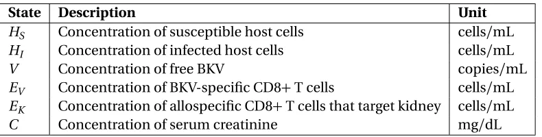
Table 2.1 Description of state variables. . . 11
Table 2.2 Description of model parameters and corresponding fixed values . . . 11
Table 3.1 Summary of cell dynamics under influence of immunosuppression. . . 32
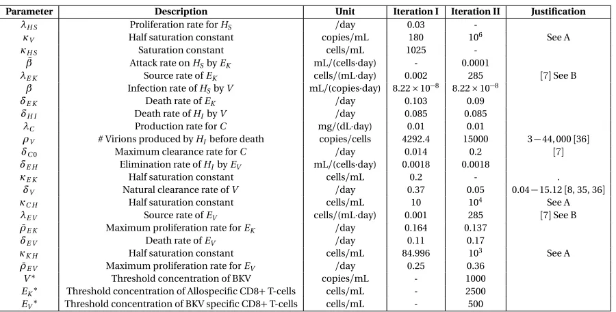
Table 3.2 Original (Iteration I) and new model (Iteration II) parameters. . . 37
LIST OF FIGURES
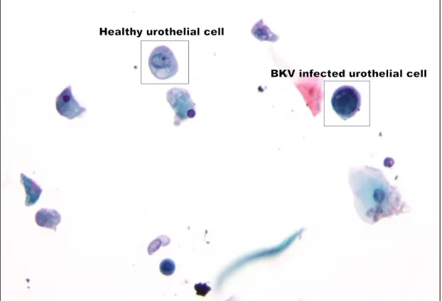
Figure 1.1 Urothelial cell infected by BKVCopyright ©2011 Michael Bonert. . . 6
Figure 2.1 Model diagram of the BKV virus affecting renal cells[8]. . . 12
Figure 2.2 Patient TOS003 BKV viral plasma loads and plasma creatinine levels. . . 13
Figure 2.3 Viral load modified pseudo errors vs. time for variousγ1values. . . 18
Figure 2.4 Creatinine modified pseudo errors vs. time for variousγ2values. . . 19
Figure 2.5 Model (2.1) solution and clinical data withγ=(0.5, 0). . . 20
Figure 2.6 Modified residuals for V and C withγ= (0.5, 0). . . 20
Figure 2.7 Model (2.7) solution and simulated data created from model (2.1) withγ=(0.5, 0). 22 Figure 2.8 Modified residuals for V and C withγ= (0.5, 0). . . 23
Figure 2.9 Model (2.1) solution and simulated data created from model (2.7) withγ=(0, 0.7). 24 Figure 2.10 Modified residuals for V and C withγ= (0, 0.7). . . 24
Figure 3.1 Schematic of the iterative modeling process[11]. . . 27
Figure 3.2 Plot illustrating the balance between under and over suppression of the im-mune response. . . 32
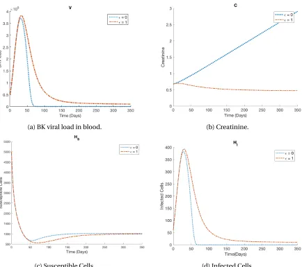
Figure 3.3 BK viral load in blood, creatinine, susceptible and infected cell dynamics for highest and lowest immunosuppressant dosages. . . 34
Figure 3.4 Model simulations for both Iteration I and II of modeling for differentεI values. 39 Figure 3.5 Figures showing the step functions used in Iteration II model (3.3) and their smooth approximations used in Iteration III model (3.5). . . 43
Figure 3.6 Model simulations for Iteration II and III of modeling for differentεI values. . 44
Figure 4.1 A sample plot showing the concept of RHC[24]. . . 54
Figure 4.2 A schematic diagram showing the RHC algorithm[24]. . . 55
Figure 4.3 Model dynamics whenεdosages are fixed. (Red dashed line is the upper bound on healthy biomarker values.) . . . 59
Figure 4.4 Open loop control for weights(WV,WC) = (1, 1)with varyingε0. . . 62
Figure 4.5 Open loop control for weights(WV,WC) = (1, 1)with varyingε0. . . 63
Figure 4.6 Open loop control with varyingWV with initial immunosuppressant,ε0=0.45. 64 Figure 4.7 Open loop control with varyingWC with initial immunosuppressant,ε0=0.45. 65 Figure 4.8 Optimal immunosuppressant dosage for first 340 days of treatment with an initial guess for control estimationε0=0.45 when perfect information is avail-able on the patient every 20 days.The blue dots are the daily recommended optimal dose. (Red dashed line is the upper bound on healthy biomarker values.) . . . 67
Figure 4.9 State estimation whenQ>>R: Filter trusts data more. . . 68
Figure 4.10 State estimation whenR>>Q: Filter trusts model more. . . 69
Figure 4.11 State estimation whenR≈Q: Current Settings. . . 69
Figure A.1 Simulated viral load modified pseudo errors vs. time for variousγ1values. . . 95
CHAPTER
1
INTRODUCTION
Abbreviations
BKV BK virus
CKD Chronic Kidney Disease
ESRD End Stage Renal Disease
GvHD Graft-Versus-Host Disease
GFR Glomerular Filtration Rate
HCMV Human Cytomegalovirus
HIV Human Immunodeficiency Virus
PVAN Polyomavirus type BK-associated Nephropathy
1.1
Thesis Outline
The rest of this chapter is dedicated to explaining the motivation, previous works and some back-ground biology for modeling immune response in renal transplant recipients. Chapter 2 explains a
method to choose the correct statistical model directly from a set of observations and then identify
any mathematical model misspecification in context to the problem defined in Chapter 1. Chapter 3 is dedicated to illustrating the iterative process of modeling biological systems by improving the
existing model introduced in Chapter 2 and making it biologically more realistic. Using the model
developed in Chapter 3, we present in Chapter 4, the algorithm and tools used in the development of an optimal treatment schedule for renal transplant recipients and the consequent results. In Chapter
5, we explore future directions in the field of renal pharmacogenomics and specific drug dynamics
of immunosuppressants as it applies to personalized medicine. A summary and conclusion is given in Chapter 6.
1.2
Motivation
According to the Organ Procurement and Transplantation Network (OPTN) as of March 11, 2018,
kidney transplants are the highest number of solid organ transplants, comprising of 428,298 trans-plants between January 1, 1988 to February 28, 2018[92]. There are currently 114,949 people waiting
for lifesaving organ transplants in the U.S. Of these, 95,301 await kidney transplants[78]. Glomerular
Filtration Rate (GFR) is often used as an indicator for kidney health and function; it measures the rate at which the kidney clears toxic waste from the blood. A GFR number of 90 or less in adults is
used as an indicator for kidney disease[30]. Chronic kidney disease (CKD), also commonly known as
chronic kidney failure, is characterized by gradual but progressive loss of kidney function. The fifth stage of CKD, called End Stage Renal Disease (ERSD), occurs when kidney function reduces to less
than 15% and leads to permanent kidney failure[30]. Patients with ESRD have two choices of therapy
- dialysis or kidney transplantation. Kidney transplantation is often chosen since transplants (grafts) can improve survival and lower healthcare costs compared to dialysis[44].
While most talk about the success rate of kidney transplants, the National Kidney foundation[91]
points out that although the official statistics is that at the the end of the first month 97% of total renal transplant recipients have a working transplant, that number decreases to 93% by the end of
the first year and becomes 83% by the end of 3 years. At 10 years, only 54% of transplant kidneys are
still working. In fact, over 20% of kidney transplants every year are re-transplants. (Note that the transplant statistics are the most recent overall numbers from the Scientific Registry of Transplant
results from a particular transplant program is available at[1].) The authors in[89]studied kidney
transplants that progressed to failure after a biopsy for clinical indications and narrowed down the top three causes for renal failure. The most prevalent cause for failure was due to organ rejection,
followed by glomerulonephritis caused in patients with infections in the throat or skin. The third
most prevalent cause for kidney rejection is polyomavirus-associated nephropathy (PVAN)(7%). PVAN is mainly caused by high-level replication of the human polyomavirus type 1, also called BK
virus (BKV), in renal tubular epithelial cells[35]. Currently there are no BKV-specific antiviral therapy,
but in some cases, BKV replication may be controlled by reducing the level of immunosuppression [48].
In order to prevent the body from rejecting the transplant, patients are usually put on a lifetime
regime of immunosuppressive medications to prevent the body from rejecting the allograft[51].
However these immunosuppressive treatments often leave the recipient susceptible to oppor-tunistic bacterial and viral pathogens and can even reactivate latent viruses preexisting in the
recipient and/or donor’s organ. Common viruses that impact transplant recipients include human
cytomegalovirus (HCMV), Epstein-Barr virus (EBV), human herpes virus (HHV)-6, HHV-7, and human polyomavirus 1 (BK virus)[8]. Thus for a renal transplant to be successful, a crucial but
fragile balance needs to be struck between over-suppression and under-suppression of the immune
system. While the former can weaken the body’s immune response making it susceptible to infec-tions, the latter can cause the immune response to fight the renal graft leading to kidney rejection.
Currently, immunosuppressive treatment protocols in the United States are in a state of flux with varying treatment regimens across different organ transplant centers. One possible reason for this
inconsistency is that centers are implementing individual or group based treatment protocols[22,
39].
The lack of consistent immunosuppressive treatment strategies across transplant centers and the narrow therapeutic index of immunosuppressants motivates us to mathematically and statistically
model dynamics of the immune system in the context of BKV infections. Our goal is to build a
robust dynamical systems model which emulates the human immune response to the allograft and BKV infection in the renal tubular epithelial cells of the transplanted kidney. We then aim to use
this model to formulate an adaptive personalized treatment strategy for renal transplant recipients
using feedback optimal control methods.
1.3
Recent Modeling Efforts in Kidney Transplantation
Several research groups have recently contributed to developing mathematical models to study
specifically kidney transplantation.
Funket al.,[37]use simple mathematical equations to investigate the relationship between BKV
replication and polyomavirus type BK-associated nephropathy (PVAN), one of the most common viral complications to develop in renal transplant recipients. It is a prominent cause of renal
transplant dysfunction and graft loss. Since PVAN was first reported in 1995, an occurrence rate
from 1% to 10% has been reported[47]. Prevalence of PVAN is mainly attributable to BK virus. The authors in[37]assume the BK virus grows and decays exponentially and then present the
corresponding equations to calculate the viral doubling times and half-lives. The generation time
and basic reproductive ratio(R0)equations are also given. The authors then perform a retrospective mathematical analysis on 15 individual patient datasets with the given equations. Their results
indicate rapid replication of the BK virus, elucidating the progressive nature of PVAN, contrary to
the general perception in clinical practice. The authors also propose the use ofR0as a measure of the efficiency of anti-viral interventions in future studies.
The authors of[35]extend this work and first perform statistical analysis on datasets from 223 kidney
transplant recipients to help understand the relationship between BKV in the plasma and urine. The
authors present a dynamical model that considers four cell populations and two virus populations: uninfected kidney tubular epithelial cells, infected tubular epithelial cells, plasma virus, uninfected
urothelial cells, infected urothelial cells, and urine virus. Antiviral interventions are represented as a time-dependent function that affects the growth of both viral populations. The basic reproductive
ratio for the kidney and urinary compartments are determined and used in parameter sensitivity
analysis. The authors simulate the mathematical model to explore the dynamics of BKV for various scenarios and compare simulation results to 7 individual kidney transplant patient datasets. The
scenario that best matches the clinical data assumes viral replication starts in the kidney, infects
urothelial cells, and then a bidirectional viral flux increases replication in both compartments. The results provide insights into the relationship between the two compartments with respect to BKV
replication and suggest further awareness into PVAN progression.
Kepleret al.,[55]also consider the effect of the immune response on the viral infection in the presence
of immunosuppression therapy. The authors specifically consider human cytomegalovirus (HCMV) infection (one of eight known human herpes viruses) in SOT recipients and present a model that
describes the dynamics of the viral load, immune response, actively-infected cells, susceptible
cells, and latently-infected cells. The authors show that the model can describe the three types of infection: primary, latent, and reactivation. Model simulations are given for varying amounts of
immunosuppression. Due to the limited amount of corresponding data in literature, the authors do
insights into the heterogeneity in disease progression.
Bankset al.,[7]modify the model in[55]to include the body’s immune response to a donor kidney. Their model considers susceptible cells, infected cells, free HCMV, HCMV-specific CD8+T-cells, allospecific CD8+T-cells that target the donor kidney, and serum creatinine, a biological marker
for renal function. Due to a lack of data, model validation is not provided; model simulations with
varying antiviral and immunosuppressive drug efficacy are produced only to verify that results match clinical trends. The authors then use simulated data to demonstrate an optimal control
problem to design an adaptive anti-viral and immunosuppressant treatment schedule that balances
over-suppression and under-suppression of the immune system. Bankset al.,[8]further modify this model to consider BKV infection and partially validate the resulting model using clinical data. Due
to the large number of parameters and limited data, the authors implement an iterative process to
identify the most sensitive model parameters to be estimated.
1.4
The Immune System and BK Virus in Context of Kidney Transplants
BK Virus was first detected in 1971 in a Sudanese kidney transplant recipient with initials “BK”[4, 17,
84]. This virus is found in over 80% of the world’s population, but infection doesn’t cause illness in
healthy immunocompetent people[4], replication of the virus often occurs during states of immune suppression[17]. BKV belongs to the polyomaviridae family which also includes JC virus (JCV)
and simian virus (SV40)[84]. BK Virus is the primary etiologic agent in most cases where patients
exhibit symptoms of PVAN, although JC virus can also cause PVAN. BK Virus is a more recently recognized viral infection that can affect the renal graft early and late after transplantation. It’s
detection and treatment are best managed in a transplantation center. It is a ubiquitous virus that
remains in a latent state. About 30% to 60% of kidney transplant recipients develop BK viruria after transplantation, and 10% to 20% develop BK viremia. Among those who develop BK viremia, 5%
to 10% develop BK nephropathy; of these, approximately 70% lose the allograft and the remainder
exhibit some kidney dysfunction. BK infection may be associated with ureteral stenosis and possible obstruction, tubulointerstitial nephritis, and a progressive rise in the serum creatinine level, with
ultimate allograft failure. Such infection must be evaluated in any episode of renal dysfunction and
prospectively evaluated approximately every 3 to 6 months in the first year after transplantation [50]. Reactivation and/or spike in BKV load in renal transplant recipients is often due to the high dosage of the potent immunosuppressants prescribed to decrease the odds of graft rejection. There is currently no approved antiviral drug therapy available to fight BKV; vigilant screening for early
detection and monitoring the immunosuppressant dosage are the only prevention methods for
Figure 1.1: Urothelial cell infected by BKV
Copyright ©2011 Michael Bonert
The immune response can be divided into two kinds, innate immune response (natural, same with each encounter) and acquired immune response (adaptive, improves on repeated exposure).
Some cells that depict innate immune response are phagocytic cells (neutrophils, monocytes,
macrophages), inflammatory mediator cells ((basophils, mast cells, and eosinophils) and natural killer cells. The acquired immune response on the other hand is responsible for the proliferation
of antigen-specific B and T cells. B cells create immunoglobulins (antigen specific antibodies responsible for eliminating foreign microorganisms). T cells help B cells to make antibodies and can
annihilate intracellular pathogens by activating macrophages and killing virally infected cells. White
blood cells (WBCs), (also called leukocytes), are the cells of the immune system that are involved in protecting the body against both infectious disease and foreign invaders. A CD8+T-cell (also
known as cytotoxic T cell or killer T-cell) is a type of white blood cell that kills cancer cells, cells that
are infected (particularly with viruses), or cells that are damaged in other ways. A CD4 T-cell (also known as mature T helper cell) is a type of WBC that sends signals to other types of immune cells,
including CD8+T-cells. All compartments of the immune system seem to be involved in keeping
pathogens like BKV at bay, virus-specifc T-cells being of particular importance[2].
As mentioned earlier in Section 1.2, Glomerular Filtration Rate(GFR) is used to measure kidney health and function[29]. The compound serum creatinine is produced as a byproduct of muscle
metabolism (breakdown of a product called phosphocreatine in the muscle) and excreted in the
as a surrogate to assess GFR. Thus the two biomarkers that can be readily measured to ascertain
CHAPTER
2
MATHEMATICAL AND STATISTICAL
MODEL MISSPECIFICATION IN
MODELING IMMUNE RESPONSE IN
RENAL TRANSPLANT RECIPIENTS
2.1
Introduction
Mathematical and statistical models are useful tools to investigate the mechanisms of any complex biological process. In Chapter 1 we introduced our problem and our motivations behind building
a mathematical model for the immune response and formulating an adaptive treatment regimen
for renal transplant recipients. In the presence of data, a statistical model is necessary to account for the discrepancy between the actual phenomenon and the observation process. In this chapter,
in context of the problem introduced in Chapter 1, we build on the work of Bankset al.,[8]and
investigate the uncertainty in clinical data from a BKV infected kidney transplant recipient.
predictions from the mathematical model, compute and plot residuals or modified residuals against
time and predictions to see if they are random. If residual plots are not randomly distributed around the horizontal axis a new statistical model is chosen and the process repeated[9]. There are two
major disadvantages of this method, first that it is time consuming and computationally expensive,
as it might take several attempts of performing an inverse problem to identify the correct statistical model associated with the observation process. Second, it determines the correct statistical model
under the tacit assumption that one has a correct mathematical model, which when modeling
complex biological systems, may not always be the case.
To overcome these drawbacks, in this chapter, we introduce a second order difference-based method to identify the correct statistical model directly from the time series data, without making any
assumptions about the accuracy of the mathematical model. After performing an inverse problem
with this appropriate statistical model, we demonstrate how modified residual or residual plots can reveal error in the mathematical model if any. The remainder of the chapter is as follows. Section 2.2
contains an overview of the BKV model and clinical data. The inverse problem and difference-based
methodologies are given in Sections 2.3 and 2.4, respectively. Section 2.5 includes our results using both clinical and simulated data. Lastly, we present our conclusions in Section 2.6.
2.2
Mathematical Model and Clinical Data
2.2.1 Mathematical Model Synopsis
We consider the following BKV model in[8], which describes the dynamics of the free BK viral load (V), susceptible cells (HS), BKV infected cells (HI), BKV-specific CD8+T cells (EV), allospecific CD8+T cells (EK), and the surrogate for GFR, serum creatinine (C)
˙ HS=λH S
1− HS
κH S
HS−βHSV (2.1a)
˙
HI=βHSV −δH IHI−δE HEVHI (2.1b) ˙
V =ρVδH IHI−δVV −βHSV (2.1c)
˙
EV = (1−εI)[λE V +ρE V(V)EV]−δE VEV (2.1d) ˙
EK = (1−εI)[λE K +ρE K(HS)EK]−δE KEK (2.1e) ˙
where
ρE V(V) = ¯ ρE VV V +κV
, (2.1g)
ρE K(HS) = ¯ ρE KHS HS+κK H
, (2.1h)
δC(EK,HS) =
δC0κE K EK +κE K ·
HS HS+κC H
, (2.1i)
and initial conditions,
(HS(0),HI(0),V(0),EV(0),EK(0),C(0)) = (HS0,HI0,V0,EV0,EK0,C0). (2.1j)
Susceptible cells proliferate logistically at a maximum rateλH S with carrying capacityκH S. Sus-ceptible cells and free virions are both lost due to interacting with each other at rateβ, resulting in infected cells. Infected cells lyse at rateδH I due to the cytopathic effect of the virus and produce pV virions. BKV-specific CD8+T cells also eliminate infected cells at rateδE H. The free virus is naturally cleared at rateδV. Both the BKV-specific CD8+T cells and the allospecific CD8+T cells are inversely related to the immunosuppressant dosage efficiencyεI. The source rates forEV and EK are given byλE V andλE K respectively. The BKV-specific CD8+T cells proliferate in the presence of free virions at maximum rate ¯ρE V with half saturation levelκV. Similarly, the allospecific CD8+T cells proliferate in the presence of susceptible cells at maximum rate ¯ρE K with half saturation level κK H. BothEV andEK die at constant ratesδE V andδE K respectively. Creatinine is produced at rateλC. The clearance rate forC is dependent upon bothEK andHSwith a maximum clearance rate ofδC0and saturation levelsκE K andκC H. The efficiency of the immunosuppressantεI is approximated by the following piecewise constant function
εI(t) =
ε1 t ∈[0, 21]
ε2 t ∈(21, 60]
ε3 t ∈(60, 120]
ε4 t ∈(120, 450].
(2.1k)
The state variable descriptions and units can be found in Table 2.1. The diagrammatic representation of model (2.1) is given in Figure 2.1. Table 2.2 contains the description of the model parameters and
fixed values. Note that these values that we treat as fixed parameters are estimated in[8]using an
Table 2.1: Description of state variables.
State Description Unit
HS Concentration of susceptible host cells cells/mL HI Concentration of infected host cells cells/mL
V Concentration of free BKV copies/mL
EV Concentration of BKV-specific CD8+T cells cells/mL EK Concentration of allospecific CD8+T cells that target kidney cells/mL
C Concentration of serum creatinine mg/dL
Table 2.2: Description of model parameters and corresponding fixed values
Parameter Description Unit Value
λH S Proliferation rate forHS 1/day 0.030
κV Saturation constant copies/mL 180.676
κH S Saturation constant cells/mL 1025.888
λE K Source rate ofEK cells/(mL·day) 0.002
β Infection rate ofHS byV mL/(copies·day) est.
δE K Death rate ofEK 1/day est.
δH I Death rate ofHI byV 1/day 0.085
λC Production rate forC mg/(dL·day) 0.007
ρV # Virions produced byHI before death copies/cells 4292.398
δC0 Maximum clearance rate forC 1/day 0.014
δE H Elimination rate ofHI byEV mL/(cells·day) 0.002
κE K Saturation constant cells/mL 0.200
δV Natural clearance rate ofV 1/day 0.372
κC H Saturation constant cells/mL 10.000
λE V Source rate ofEV cells/(mL·day) 0.001 ¯
ρE K Maximum proliferation rate forEK 1/day est.
δE V Death rate ofEV 1/day est.
κK H Saturation constant cells/mL 84.996
¯
ρE V Maximum proliferation rate forEV 1/day est. εI Efficacy of immunosuppressive drugs
2.2.2 Log-scaled Model
Due to a scale difference among model states and model parameters as well as to ensure that state
variables do not become negative, we use log transformation to resolve any scaling issues during
numerical simulations and implementation of the inverse problem (see[8]for details). We can rewrite model (2.1) as the vector system,
dy
Figure 2.1: Model diagram of the BKV virus affecting renal cells[8].
where
y= [HS,HI,V,EV,EK,C]T,
q= [λH S,λE K,λE V,λC,β,δE H,δV, ¯ρE V,δE V,δE K,δC0,δH I,κC H,κK H,κH S,κE K,κV,ρV, ¯ρE K, ε1,ε2,ε3,ε4]T,
and
y(0) =y0.
We make the afore-mentioned log transformation by defining variables
xi=log10(yi), i=1, 2, 3, 4, 5 x6=y6,
x0i=log10(y0i), i=1, 2, 3, 4, 5 x06=y06,
Then the log-scaled model becomes
dx
d t =g(x,q,x0), wheregi(x,q,x0)is given by
gi(x,q,x0) =
d xi d t =
d xi d yi
d yi d t =
1 yil n(10)
hi(y,q,y0), i=1, 2, 3, 4, 5
= 1
10xil n(10)hi(10
(x1,x2,...,x5),x
6, 10(q1,q2,...,q19),q20,q21, . . . ,q23, 10(x01,x02,...,x05),x06),
and
g6(x,q,x0) =h6(y,q,y0)
=h6(10(x1,x2,...,x5),x6, 10(q1,q2,...,q19),q20,q21, . . . ,q23, 10(x01,x02,...,x05),x06).
2.2.3 Clinical Data
We investigate uncertainty in the clinical data[8]. This data set consists of eight BK viral plasma
load (DNA copies/mL) measurements and sixteen plasma creatinine level (mg/dL) measurements
for patient TOS003 from Massachusetts General Hospital. The patient was diagnosed with BKV infection in the first 3 months of transplantation. With every visit, dosage and combination of
immunosuppressants were updated. Figure 2.2 contains the plots of the data.
(a) BK viral load data (b) Creatinine data
2.3
Inverse Problem Method and Statistical Model Selection
We follow standard inverse problem procedures to estimate parameters in our mathematical model [9, 11, 25, 88]. Consider a generalN-dimensional dynamical system with parameter vectorq,
dx
d t (t) =g(t,x(t);q), x(t0) =x0,
with anmdimensional observation process
f(t;θ) =Cx(t;θ),
whereθ= (qT,xT0)Tis the vector of parameters along with the initial conditions to be estimated andC is them×N observation matrix.
Our data set consists of observed values for the plasma viral load and creatinine levels. Thus our observation matrix is the following
C =
0 0 1 0 0 0 0 0 0 0 0 1
,
asx= [log10HS, log10HI, log10V, log10EV, log10EK,C]T andf= [log10V,C]T.
Letyi1represent the free BK viral load measurements andyj2represent the plasma creatinine load measurements at time pointsti1,i =1, 2, . . . ,n1and tj2,j =1, 2, . . . ,n2respectively. Heren1 =8 andn2=16. We note that there is some discrepancy between the actual phenomenon, which is
represented through the data, and the above observation process. We account for this uncertainty with the statistical models,
Yi1=f1(ti1;θ0) +f1(ti1;θ0)γ1Ei1, i=1, 2, . . . ,n1,
Yj2=f2(tj2;θ0) +f2(t2j;θ0)γ2Ej2, j=1, 2, . . . ,n2,
whereγ≥0and thep×1 vectorθ0∈Ωis the “true” or nominal parameter set. Here f1(ti1;θ0) =
x3(ti1;θ0)andf2(tj2;θ0) =x6(ti2;θ0). Then1×1 andn2×1 random error vectorsE1andE2respectively
and Var(Ej2) =σ202. The corresponding realizations are,
yi1=f1(ti1;θ0) +f1(ti1;θ0)γ1ε1i, i=1, 2 . . . ,n1,
y2j=f2(tj2;θ0) +f2(tj2;θ0)γ2ε2j, j=1, 2 . . . ,n2.
This multiplicative structure of the observational error in the above statistical model exists because
often in biological models the size of the observation error is proportional to the size of the observa-tions. Forγ≥0, a generalized least squares method or an iterative weighted least squares method as used below is appropriate to perform the inverse problem. In order to estimateθ0, we want to
minimize the distance between the collected data and mathematical model, where the observables are weighted according to their variability and, for each observable, the observations over time are
weighted unequally.
The iterative weighted least squares estimateθˆI W LSis numerically determined by iteratively solving the following system :
ˆ
θI W LS=argmin
θ∈Ω
n1 X
i=1
[yi1−f1(ti1;θ)] T ˆ
V1−1(ti1)[yi1−f1(ti1;θ)] (2.2)
+
n2 X
j=1
[yj2−f2(t2j;θ)]TVˆ2−1(tj2)[yj2−f2(tj2;θ)]
ˆ V1(ti1) =
ˆ ω1
i n1−p
n1 X
i=1
(yi1−f1(ti1;θˆI W LS))2 ˆ
ω1
i
(2.3)
ˆ V2(tj2) =
ˆ ω2
j n2−p
n2 X
j=1
(y2
j −f2(tj2;θˆI W LS))2 ˆ
ω2
j
, (2.4)
where ˆω1i=f1(ti1,θˆI W LS)2γ1and ˆω2j =f2(tj2,θˆI W LS)2γ2. We use the following iterative procedure[9, 11, 25, 88]:
1. Estimateθˆ(I W LS0) using (2.2) with ˆV1(ti1) =1 and ˆV2(t2j) =1. Set k=0. 2. Compute weights ˆω1i(k)=f1(ti1,θˆ
(k)
I W LS)2γ1 and ˆω
2(k)
j =f2(t2j,θˆ (k) I W LS)2γ2. 3. Solve for ˆV1(t1
i) (k)
and ˆV2(t2
j) (k)
usingθˆI W LS(k) , ˆωi1(k), and ˆω2j(k)in equations (2.3) and (2.4) re-spectively.
4. EstimateθˆI W LS(k+1) using ˆV1(ti1) (k)
and ˆV2(tj2) (k)
5. Setk:=k+1 and return to step 2. Terminate when two successive estimates forθˆI W LSare sufficiently close.
Note that this is not the same as taking the derivative of the argument in the right side of (2.2) and setting it equal to zero. For more details see page 63 of[9]and page 89 of[88].
The estimated variances for each observableσ2
01andσ022 are approximated by the following:
ˆ σ2
01=
1 n1−p
n1 X
i=1
y1
i −f1(ti1;θˆI W LS) f1(ti1;θˆI W LS)γ1
2
ˆ σ2
02=
1 n2−p
n2 X
j=1
y2
j −f2(tj2;θˆI W LS) f2(tj2;θˆI W LS)γ2
2
.
If we assumeγ= (γ1,γ2) = (0, 0), then our statistical model is called an absolute error model and an
ordinary least squares method is appropriate for parameter estimation. Bankset al.[8]consider an absolute error model and additionally assume that the variances for each observable are equal
(i.e.,σ201=σ202). While the statistical model choice in[8]yields good results, we believe it is more biologically realistic to assume the variance in observation errors are not equal and the size of the
observation error is proportional to the size of the observed quantity.
2.4
Difference-based Methods and Modified Residuals
We use a second order difference-based method to determine the correct statistical model (γγγvalue) [6, 13]. Another method often implemented consists of performing an inverse problem with someγγγ value and computing the modified residuals
Mk l=
ylk−fk(tlk;θˆ) fk(tlk;θˆ)γk
, (2.5)
for each observablek at timetl,l =1, . . . ,nk. The plots ofMk l vs.tl should be randomly scattered around the horizontal axis. If an undesired non-random shape is present (e.g., a megaphone or
inverted megaphone shape), then a differentγγγvalue is chosen and the process is repeated until aγγγvalue produces the desired random scatter plot. However, this method does not consider both the mathematical model and statistical model misspecifications; it determines the correct
may be computationally expensive) and plotting the modified residuals until a good statistical
model is chosen.
We follow[6]and first apply the second order difference-based method directly to the data to determine the correctγγγvalue, which is both computationally economical as well as time efficient and independent of any assumed correct mathematical model. We first calculate the following
pseudo measurement errors for observablekat timetl,l=1, . . . ,nk
ˆ εk l = 1 p
2(y k l+1−y
k
l ) forl=1
1
p
6(y k l−1−2y
k l +y
k
l+1) forl=2, . . . ,nk−1
1
p
2(y k l −y
k
l−1) forl=nk.
Next we calculate the modified pseudo errors
ηk l =
ˆ εk
l
|ylk−εˆkl|γk
for observablek at timetl,l=1, . . . ,nkfor different values ofγk. (For derivation of modified pseudo errors see Appendix A.1.) We plot these modified pseudo errors vs. time for differentγkvalues to find theγk value that produces a random scatter plot. Once the correct observational error is accounted for, we perform the inverse problem with this statistical model and compute the modified residuals in (2.5). If the modified residual plots are not randomly distributed around the horizontal axis, then
the error must be due to mathematical model misspecification, implying another iteration of the
modeling process is needed. Note that just using modified residuals is insufficient in detecting mathematical model misspecification; using modified pseudo errors in combination with modified
residuals as described above would assist in identifying any discrepancies in mathematical model
2.5
Results
2.5.1 Clinical Data
Using second order differencing, we plot the modified pseudo errors for both viral load and creatinine versus time and visually assess the plots to choose an appropriateγvalue. Figure 2.3 contains the graphs of the viral load modified pseudo errors vs. time for variousγ1values. As can be seen due to
the limited amount of data, it is difficult to determine the correctγ1value through visual assessment.
The valueγ1=0.5 provides an approximately symmetric distribution around the horizontal axis with
relatively small modified pseudo error values. The creatinine modified pseudo errors for different γ2values are given in Figure 2.4. The modified pseudo errors withγ2=0 appear to be randomly
distributed whereas the modified pseudo errors withγ2=1 reveal a slight non-random (megaphone)
shape. Even though we visually assess the plots to pick a suitableγvalue to the best of our ability, the sparseness of the data set makes it difficult to make a stronger case for a particular statistical
model.
(a)γ1=0 (b)γ1=0.5
(c)γ1=1
Figure 2.3 (cont.): Viral load modified pseudo errors vs. time for variousγ1values.
(a)γ2=0 (b)γ2=1
Figure 2.4: Creatinine modified pseudo errors vs. time for variousγ2values.
With our best guess of the correct statistical model,γ= (0.5, 0), we next perform an inverse prob-lem for the 5 most sensitive parameters[8]and obtain the modified residuals in order to detect
the presence of mathematical model error. We perform the inverse problem using the MATLAB
function
fmincon
. The initial guesses for the parameters are those used in[8]and lower and upper bounds are set for each of the 5 parameters for computational efficiency. The estimated parameters,resid-uals in Figure 2.6 appear to form a random band around the horizontal axis. This suggests that the
mathematical model accurately describes the biological process, although again it is difficult to conclude this with conviction due to the limited amount of data.
(a) BK virus model solution and data (b) Creatinine model solution and data
Figure 2.5: Model (2.1) solution and clinical data withγ=(0.5, 0).
(a) Modified residuals for BK virus (b) Modified residuals for creatinine
2.5.2 Simulated Data
When using the second order difference-based method with sparse clinical data, it is not very easy to pick a statistical model or make a strong case for the presence/absence of mathematical model misspecification. To illustrate the need for a denser data set, we repeat the above process with the
following simulated data created by adding noise to the “true” model solution
Vi=f1(ti1;θ0) +f1(ti1;θ0)γ1ε1
i, (2.6a)
Cj=f2(tj2;θ0) +f2(tj2;θ0)γ2ε2j, (2.6b)
whereE1∼N(0, 0.3),E2∼N(0, 0.03),γ= (0.5, 0), and the estimated parameters
[log10β, log10ρ¯E V, log10δE V, log10δE K, log10ρ¯E K] = [−7.067,−0.601,−0.964,−0.995,−0.785]. We as-sume that “data" is collected every week forttt1=ttt2= [0, 7, 14, ..., 448]. As expected, the second order differencing method produces the desired scatter plot forγγγ= (0.5, 0)and undesired megaphone shapes for otherγγγvalues (see Appendix A.2 for corresponding figures). The modified residual plots also exhibit no mathematical model misspecification, which is expected since the data was created
using the mathematical model (see Appendix A.3 for modified residual plots).
We now demonstrate how the modified residual plots can detect mathematical model error or misspecification by performing an inverse problem with a simpler version of model (2.1), given in
(2.7). While the original model (2.1) assumes the susceptible population grows logistically where
cell proliferation and the eventual plateauing of the population is dependent on the susceptible population size, the simpler model (2.7) assumes a growth rate ofλH S−δH SHS, whereHScells are produced at a constant rateλH S (cells/(mL·day)) independent of the cell population and die at a rate proportional toHSwith a proportionality constant or death rate ofδH S(1/day). The simpler model is given by the following
˙
HS=λH S−δH SHS−βHSV (2.7a)
˙
HI=βHSV −δH IHI−δE HEVHI (2.7b) ˙
V =ρVδH IHI−δVV −βHSV (2.7c)
˙
EV = (1−εI)[λE V +ρE V(V)EV]−δE VEV (2.7d) ˙
EK = (1−εI)[λE K +ρE K(HS)EK]−δE KEK (2.7e) ˙
where
ρE V(V) = ¯ ρE VV V +κV
, (2.7g)
ρE K(HS) = ¯ ρE KHS HS+κK H
, (2.7h)
δC(EK,HS) =
δC0κE K EK +κE K ·
HS HS+κC H
, (2.7i)
and initial conditions,
(HS(0),HI(0),V(0),EV(0),EK(0),C(0)) = (HS0,HI0,V0,EV0,EK0,C0). (2.7j)
The immunosuppressant efficiency is defined by the piecewise constant function (2.1k).
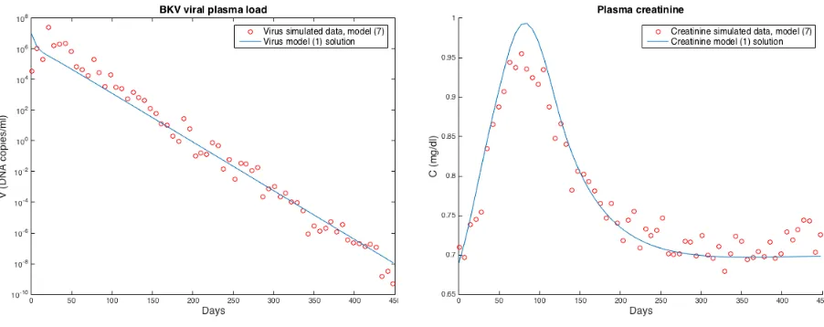
We perform the inverse problem usingγγγ= (0.5, 0)to estimate the 6 parametersβ, ¯ρE V,δE V,δE K, δH S, ¯ρE K and obtain the solutions in Figure 2.7. The estimated parameters,[log10β,log10ρ¯E V, log10δE V,log10δE K,log10δH S,log10ρ¯E K] = [−7.061,−0.632,−0.632,−1.007,−0.92,−0.704]. Even though the simpler model produces a reasonable fit to the data, the modified residuals produce
a strong non-random pattern (Figure 2.8). Since we already eliminated statistical error model
discrepancy (through the difference-based method), these non-random modified residuals indicate a mathematical model misspecification. That is, the simpler model (2.7) is unable to accurately
capture the dynamics represented in the data.
(a) BK virus model solution and simulated data (b) Creatinine model solution and simulated data
(a) Modified residuals for BK virus (b) Modified residuals for creatinine
Figure 2.8: Modified residuals for V and C withγ= (0.5, 0).
We next investigate mathematical model misspecification when a more complex model than
war-ranted is assumed. To do so, we create a new simulated data set fort1=t2= [0, 7, 14, . . . , 448]using (2.6) wheref1andf2now represent log10V andCin model (2.7),γγγ= (0, 0.7),E1∼N(0, 0.5), andE2∼
N(0, 0.02). Parameter values from Table 2.2 are used to create the new simulated data set with free pa-rameters[log10β,log10ρ¯E V,log10δE V,log10δE K,log10ρ¯E K]= [−7.067,−0.601,−0.964,−0.995,−0.785] and additional parameterδH S=0.003/day[35].
As expected, the difference-based method withγγγ= (0, 0.7)produces random scatter plots (see Appendix A.3). We perform the inverse problem with this data set and the original model (2.1). The
estimate values for the 5 parameters are,[log10β, log10ρ¯E V,log10δE V,log10δE K, log10ρ¯E K]=[−8.020,
−0.744,−0.223,−0.863,−0.675]. The model (2.1) solutions and corresponding modified residu-als are plotted in Figure 2.9 and Figure 2.10. Even though the fit between the model and data
looks acceptable, the modified residuals display a strong non-random pattern, indicating incorrect
(a) BK virus model solution and simulated data (b) Creatinine model solution and simulated data
Figure 2.9: Model (2.1) solution and simulated data created from model (2.7) withγ=(0, 0.7).
(a) Modified residuals for BK virus (b) Modified residuals for creatinine
Figure 2.10: Modified residuals for V and C withγ= (0, 0.7).
2.6
Conclusion
We investigate mathematical model and statistical model misspecifications in the context of least
squares methodology using a BKV model and both clinical and simulated data. Bankset al.,[8]use ordinary least squares techniques to perform an inverse problem with clinical data. We build on
consider different variances for different observables and allow the error to depend on the size of the
observables (measurements). We follow[6]and demonstrate how difference-based methods can be applied directly to data to determine the correct statistical model and further, we illustrate the use
of modified residuals to detect mathematical model discrepancy. The presence of mathematical
model error suggests possibly another iteration of modeling might be needed. However, due to the limited amount of clinical data, no strong conclusion can be reached.
We thereby demonstrate these methods using dense simulated data. We first create data using
the BKV model (2.1) with an associated statistical model. The difference-based method correctly
identifies the assumedγvalue. Using this statistical model, we perform an inverse problem using a simpler model (2.7) where the nonlinearity is removed from the susceptible cell population growth
dynamics. While the model (2.7) solution fits the data reasonably well, the modified residual plots
depict a strong pattern, identifying the mathematical model discrepancy. We then repeat the process by creating data using the simpler model (2.7) and perform an inverse problem with the original
model (2.1). That is, we now assume a more complex dynamical system in comparison to the
biological process represented by the data. Again, the modified residuals indicate error in the mathematical model. Therefore this method can reveal mathematical model misspecification when
either simpler or more complex models are assumed as compared to the data dynamics.
Previously, modified residual plots were solely used to determine the correct statistical model by iteratively performing multiple inverse problems until the correct statistical model was chosen [9]. Using both the difference-based method as well as modified residual plots is computationally more efficient; the difference-based method can be applied directly to the data and thus multiple inverse problems need not be performed. However, and even more notably, the previous method
(using only modified residual plots) determines the statistical model under the possibly uninformed
assumption of a correct mathematical model; the use of both the difference-based method and modified residuals accounts for both types of error in the inverse problem without prior model
CHAPTER
3
IMMUNOSUPPRESSANT TREATMENT
DYNAMICS IN RENAL TRANSPLANT
RECIPIENTS: AN ITERATIVE MODELING
APPROACH
3.1
Introduction
A patient undergoing a solid organ transplantation is usually put on a lifetime regime of immuno-suppressive medications to prevent the body from rejecting the allograft[51]. However, these
immunosuppressive treatments often leave the recipient susceptible to opportunistic pathogens
including viruses. Achieving the delicate balance between under-suppression and over-suppression of the immune system is key to successful and sustainable transplantation. Mathematical and
statistical models can be important and beneficial tools that contribute to the improvement and
optimization of treatment protocols. Modeling of any biological process is an iterative one, as seen in Figure 3.1. The biologist first presents a research question about some biological process as well
as knowledge about biological relationships and mechanisms, often depicted by a schematic or
a mathematical model. Analytic or numerical analysis of the model produces results which are
in-terpreted and compared to the biological system, possibly leading to a change in the understanding of the biological relationships. The process is continuously repeated, sometimes through multiple
research efforts, using the resulting biological insights (See[11]for more details on the iterative
process of modeling).
In this chapter we first explain and analyze the exisiting model (2.1) seen in Chapter 2 which captures the biological mechanisms of the immune response in renal transplantation patients with respect
to infection caused by the human polyomavirus type 1, named “BK virus” (BKV)[8]. Our results
show evidence of the lapses in biological understanding and implementation of the corresponding mathematical model. We then attempt to address and correct for the discrepancies between the
mathematical model and the biological system by revising components of the mathematical model,
thereby illustrating the iterative process of modeling. Once a mathematical model is developed, it could in turn be used for control theory applications to predict optimal drug regimens, an important
problem we will address in the coming chapters.
3.2
Iteration I: Preliminary Model
3.2.1 Data Collection and Biological Model
Data used to fit the model and obtain some of the model parameters in[8]was collected at Mas-sachusetts General Hospital from a renal transplant patient TOS003 diagnosed with BKV in the first
3 months of kidney transplantation. (This data was collected with approval of the MGH human
subjects (IRB) committee. Furthermore data was shared with NCSU in a de-identified manner.) Eight BK viral plasma load (DNA copies/mL) measurements and sixteen plasma creatinine level
(mg/dL) measurements were collected (See Chapter 3, Figure 2.2 for plot of datasets). Creatinine
levels are used as a surrogate for GFR (Glomerular Filtration Fate), to measure kidney function. Due to the sparsity of data collected, we do not estimate parameters for Iteration II and Iteration III of
our modeling efforts, instead we use most of the parameters from literature.
The authors in[8]describe a model schematic of the compartmentalized biological model as shown in Figure 2.1 in Chapter 2.
Since no effective anti-viral treatment exists for BKV, the authors in[8]modify the model in[7]to
only consider the efficiency of immunosuppressant treatment. Additionally, the authors model the effect of the susceptible cells on creatinine clearance and on the allospecific CD8+T-cell population growth. As opposed to Funk et al.[35], the authors in[8]do not consider the urothelial cells and only
consider infection in tubular epithelial cells, in part due to the availability of data. While this makes
the model more specific, one can hope to expand the current model scope to include urothelial cells once relevant data becomes available.
3.2.2 Mathematical Model
˙ HS=λH S
1− HS
κH S
HS−βHSV (3.1a)
˙
HI=βHSV −δH IHI−δE HEVHI (3.1b) ˙
V =ρVδH IHI−δVV −βHSV (3.1c)
˙
EV = (1−εI)[λE V +ρE V(V)EV]−δE VEV (3.1d) ˙
EK = (1−εI)[λE K +ρE K(HS)EK]−δE KEK (3.1e) ˙
C=λC −δC(EK,HS)C, (3.1f)
where
ρE V(V) = ¯ ρE VV V +κV
, (3.1g)
ρE K(HS) = ¯ ρE KHS HS+κK H
, (3.1h)
δC(EK,HS) =
δC0κE K EK +κE K ·
HS HS+κC H
. (3.1i)
The initial conditions are given by,
(HS(0),HI(0),V(0),EV(0),EK(0),C(0)) = (HS0,HI0,V0,EV0,EK0,C0). (3.1j)
εI(t) =
ε1 t ∈[0, 21]
ε2 t ∈(21, 60]
ε3 t ∈(60, 120]
ε4 t ∈(120, 450].
(3.2)
Detailed explanation of the dynamics of the model and model states can be found in Subsection
3.2.3 Statistical Error Model
The authors in[8]assume the simplest statistical error model, an absolute error model, where the
variances of the error for each observable (viral load and creatinine) are equal and constant over time. That is, the authors account for the uncertainty in the dataset by the following statistical error
model
Yi1=f1(ti1;θ0) +Ei1, i=1, 2, . . . ,n1, Yj2=f2(t2j;θ0) +Ej2, j=1, 2, . . . ,n2.
The functionsf1(ti1;θ0)andf2(tj2;θ0)represent the model solution for viral load and creatinine at
timesti1andtj2respectively, assuming a “true" or nominal parameter setθ0. The existence of this
“true" parameter set is a standard assumption in statistical models[9].
TheEi1,Ej2terms represent the measurement error that causes the measurements to differ from the model solution with the “true" parameter set. We assume then1×1 andn2×1 random vectorsEi1 andE2
j respectively, are independent and identically distributed with mean zero andV a r(Ei1) = σ2
01andV a r(E 2
j) =σ202. The authors in[8]assumeσ201=σ022 (Note the model is log scaled as
shown in Chapter 2). The corresponding method for parameter estimation is ordinary least squares
(OLS).
In Chapter 2, we build on the works of[8]and consider a more general (and possibly more biologically realistic) statistical error model[13]. We assume the variances of observation errors are not equal
and allow for the errors to depend on the size of the observed quantity. That is, we assume the
following statistical error model, a relative error model, given by
Yi1=f1(ti1;θ0) +f1(ti1;θ0)γ1Ei1, i=1, 2, . . . ,n1,
Yj2=f2(tj2;θ0) +f2(t2j;θ0)γ2Ej2, j=1, 2, . . . ,n2,
forγk≥0,k =1, 2. The measurement error term now can depend on the size of the model solution of the observables. Note that if bothγ1=0 andγ2=0, the two statistical error models are equivalent. The corresponding method, for parameter estimation, assuming a relative error model is iterative
weighted least squares (IWLS).
Recall in Chapter 2, we use a second order difference-based method to eliminate statistical error model misspecification by selecting the correct statistical error model directly from the data. We
![Figure 2.1: Model diagram of the BKV virus affecting renal cells [8].](https://thumb-us.123doks.com/thumbv2/123dok_us/1664231.1209013/24.612.171.465.75.320/figure-model-diagram-bkv-virus-affecting-renal-cells.webp)


![Figure 3.1: Schematic of the iterative modeling process [11].](https://thumb-us.123doks.com/thumbv2/123dok_us/1664231.1209013/39.612.149.485.339.546/figure-schematic-iterative-modeling-process.webp)