A Study of the Errors of the Fixed-Node Approximation in Diffusion Monte Carlo.

(1)

ABSTRACT

RASCH, KEVIN M. A Study of the Errors of the Fixed-Node Approximation in Diffusion Monte Carlo. (Under the direction of Lubos Mitas.)

Quantum Monte Carlo techniques stochastically evaluate integrals to solve the

many-body Schrödinger equation. QMC algorithms scale favorably in the number

of particles simulated and enjoy applicability to a wide range of quantum systems.

Advances in the core algorithms of the method and their implementations paired

with the steady development of computational assets have carried the applicability of

QMC beyond analytically treatable systems, such as the Homogeneous Electron Gas,

and have extended QMC’s domain to treat atoms, molecules, and solids containing as

many as several hundred electrons.

FN-DMC projects out the ground state of a wave function subject to constraints

imposed by our ansatz to the problem. The constraints imposed by the fixed-node

Approximation are poorly understood. One key step in developing any scientific

theory or method is to qualify where the theory is inaccurate and to quantify how

erroneous it is under these circumstances.

I investigate the fixed-node errors as they evolve over changing charge density,

system size, and effective core potentials. I begin by studying a simple system for

which the nodes of the trial wave function can be solved almost exactly. By comparing

two trial wave functions, a single determinant wave function flawed in a known way

and a nearly exact wave function, I show that the fixed-node error increases when

the charge density is increased. Next, I investigate a sequence of Lithium systems

increasing in size from a single atom, to small molecules, up to the bulk metal form.

(2)

correlation energy of the system. Given this accuracy, I make a prediction for the

binding energy of Li4 molecule. Last, I turn to analyzing the fixed-node error in first

and second row atoms and their molecules. With the appropriate pseudo-potentials,

these systems are iso-electronic, show similar geometries and states. One would expect

with identical number of particles involved in the calculation, errors in the respective

total energies of the two iso-electronic species would be quite similar. I observe,

instead, that the first row atoms and their molecules have errors larger by twice or

more in size. I identify a cause for this difference in iso-electronic species. The

fixed-node errors in all of these cases are calculated by careful comparison to experimental

results, showing that FN-DMC to be a robust tool for understanding quantum systems

(3)

c

(4)

A Study of the Errors of the Fixed-Node Approximation in Diffusion Monte Carlo

by

Kevin M. Rasch

A dissertation submitted to the Graduate Faculty of North Carolina State University

in partial fulfillment of the requirements for the Degree of

Doctor of Philosophy

Physics

Raleigh, North Carolina

2012

APPROVED BY:

Marco Buongiorno-Nardelli Jerry L. Whitten

David Brown Lubos Mitas

(5)

DEDICATION

To my wife for patiently and tirelessly encouraging me whenever my convictions

waned while I pursued my “impulse of delight.”

To my father for encouraging me to find everything’s cause (by never answering me

with, “Because I said so.")

To my mother for gifting me with both a refusal to quit and a careful attention to

(6)

BIOGRAPHY

. . .

Nor law, nor duty bade me fight,

Nor public men, nor cheering crowds,

A lonely impulse of delight

drove to this tumult in the clouds;

(7)

ACKNOWLEDGEMENTS

I would like to thank my advisor, Dr. Lubos Mitas. He has continually challenged

my abilities and pushed me to grow as a researcher and physicist. I could not have

completed this dissertation without his support. Lubos’ enthusiasm for our research,

for educating and inspiring the next wave of students, and for science itself has

infected me, and I hope to carry that infection forward until we are all “sick” with

our love of understanding.

I would like to thank Dr. Jindrich Kolorenc, who has shown me an infinitude of

patience as I have shed the husk of a naive fresh student drunk on his ability to solve

homework problems. Jindra’s continual search for a simple, insightful perspective

and his high standard for proof will forever serve as a benchmark for “doing it right.”

I expect to ask myself many times over the coming years, “Is this enough evidence to

convince Jindra?”

I would like to thank Dr. Michal Bajdich. Michal was eternally welcoming,

considerate, and completely honest at the same time. My transition into the physics

world would have certainly been rockier if it weren’t for Michal’s advice and example.

I would like to thank Shuming Hu. During my graduate work, Shuming and I

shared an office and many, many afternoons of conversation which have profoundly

shaped my perspectives. Of all the trappings of graduate school, I will miss most of

all our laughter-filled “debates” on the nature of things.

I would like to thank Donald Jeffry Herbert (Mr. Wizard), Stephen Robert Irwin

(The Crocodile Hunter), and William Sanford Nye (the Science Guy). I would never

have cared to come this far if it weren’t for their influence. All too often becoming

(8)

others’ judgement. Each of these people has been insightful enough to recognize our

shared responsibilities and courageous enough to publicly share their passion and

encourage it in others.

I would like to thank Sue Dennis. As a member of her English class in 6th,

7th, and 8th grades, I felt something I had never felt before: the pleasure of being

respectfully treated as an intelligent and decent person. This had a profound effect on

my self-worth, for which I will be eternally grateful.

I would like to thank Susan Smith. She gave her time to be the coach of nearly

every extra-curricular science activity at Newnan High School and, by example, taught

me a competitive enthusiasm that epitomizes the spirit of proudly doing your best

work. Additionally, in her chemistry classes I encountered two things that would stay

with me and drive me to this place. Mrs. Smith’s philosophy for discipline was to

simply keep a student so busy that there was no time for horseplay–this was the first

time I can recall having to “work.” And I will never forget the colored side box in

the chemistry textbook explaining where electron orbitals come from. It was there

that I saw the Schrödinger equation for the first time. The pictures and ideas that I

encountered in that class have occupied the majority of my curiosity, and for that I

owe Mrs. Smith the thanks that a blissfully happy couple owes to the person that

(9)

LIST OF TABLES

Table 3.1 Computational efficiency for different complexity Jastrow factors in units of statistical samples per wall clock second, given in Eqn. (2.20). . . 73

Table 6.1 FNDMC ground state energies forΨHFandΨ2-confwave functions

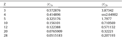
compared to the exact energies estimated from experiments for Z=4 through 28 and extrapolation to infinite basis set for Z=3. . . 93 Table 6.2 Expectation values of radiushrifor one-particle numerical

Hartree-Fock orbitals given in Bohrs. . . 93

Table 7.1 Comparison of theoretical results for the total energy of a lithium atom. . . 96 Table 7.2 Comparison of the latest calculation and measurement with

FN-DMC results for the Electron Affinity for lithium in Hartrees. The single det. result uses the single determinant result and multi-det., the multi-determinant values for Li− from Table 6.1 . . . 97 Table 7.3 FN-DMC total energy for trial wave functions from different levels

of theory testing unoptimized nodal surfaces for use as DMC trial wave functions. . . 100 Table 7.4 FN-DMC results for different basis sets with trial wave functions

from CI-SD calculations using 15 virtual orbitals and then opti-mized in with respect to VMC total energy. . . 101 Table 7.5 Summary of the optimized geometry parameters ofD2h Li4tested

in this work, and the FN-DMC total energy for each. The trial wave function is an VMC energy optimized CI-SD expansion with 93 CSFs. . . 101 Table 7.6 Binding Energies uncorrected for zero-point motion are given in

units ofeV per atom . . . 103 Table 7.7 Results for the Γ-point wave function of an 8 atom supercell

comparing the nodal quality of select DFT functionals. . . 104 Table 7.8 Summary of the exact energy per atom of a sequence of different

size Li systems estimated in the spirit of Filippi and Umrigar.

Etot for n = 4 crystal structure substitutes the ZPVE corrected

FN-DMC value for the binding energy. . . 107

(13)

Table 8.2 A comparison of FN-DMC total energies of first and second row atoms and molecules with CCSD(T) extrapolations to infinite basis size and FN-DMC results from the literature. . . 110

Table 9.1 Energy components as percentages of the total energy in Coulom-bic systems . . . 131 Table 9.2 Energy components for two- and four-electron atoms: standard

expectations and nda values . . . 134 Table 9.3 Energy components for 2p2 states for Coulomb potential:

stan-dard expectations and nda values . . . 135

(14)

LIST OF FIGURES

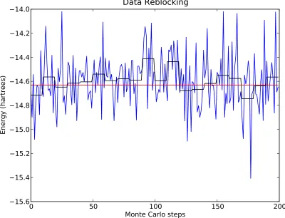
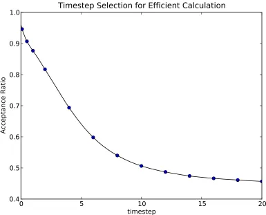
Figure 2.1 A graphical depiction of data reblocking. The blue curve repre-sents the energy of a Beryllium atom at each Monte Carlo step. The black curve represents the value of each block average over 10 steps. The red line is the final average over the entire simula-tion (longer than depicted). Notice that the values of the block average fluctuate about the mean much less than the individual step values. . . 31 Figure 2.2 The acceptance ratio for proposed moves as a function of timesteps

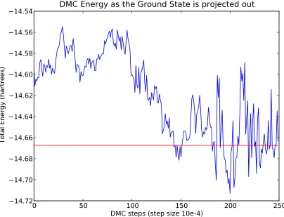
for the VMC calculation of the energy of a beryllium atom. . . . 33 Figure 2.3 The initial equilibration of a DMC calculation of a Beryllium

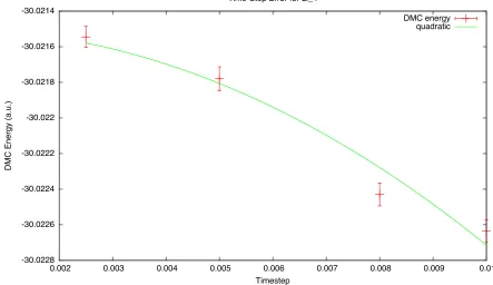
atom. The DMC energy falls as the higher energy excited states present in the trial wave function are damped by the Green’s Function. By the last 50 steps shown the simulation is equili-brated and goes on for many hundreds more steps. The final average over the entire simulation is show in red. . . 41 Figure 2.4 The exact DMC energy extrapolated to τ =0 for a Li4molecule

using an re-optimized trial wave function taken from a Configu-ration Interaction calculation. . . 47

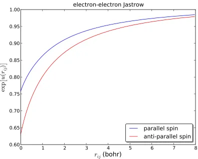
Figure 3.1 Variationally optimized e-e Jastrow factor for parallel and anti-parallel spin electrons in the case of a beryllium atom. Note the difference in the slope of each atrij =0. . . 69

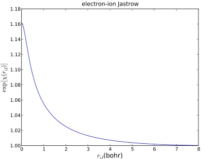
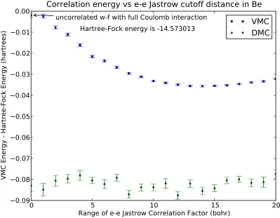
Figure 3.2 Variationally optimized electron-ion Jastrow factor in the case of a beryllium atom. The single particle orbitals satisfy the cusp conditions in this case so this Jastrow has a slope of 0 atr =0. . 70 Figure 3.3 The correlation energy of a single determinant Beryllium wave

function as a function of the cutoff distance of the electron-electron Jastrow terms. The energies shown are relative to the Hartree-Fock energy. Data depict the effect of explicit correlation in the wave function on the correlation energy. As the reach of the Jastrow factor approaches the optimal value ofrcut ≈14 bohr,

(15)

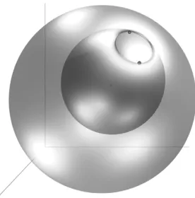
Figure 6.1 A comparison of the FNDMC error for different wave functions calculated using values in Table 6.1. The squares correspond to the HF nodes while the circles correspond to the 2-configuration nodes. The linear fit to the error from the HF nodal structure has a slope of 0.0111(1). The error bars are much smaller than the plot symbols. . . 93 Figure 6.2 3D subspace of the 2-configuration nodal surface in real space.

The two dots at the opening represent the spin-up and -down electrons fixed at slightly different radial distances. The tiny dark spot in the middle is the nucleus. The node is found by scanning the space with the remaining two electrons located on the top of each other and plotting the wave function’s zero isosurface. 3 lighting sources are used to make the curvature of the surface visible. The semi-transparency enables to see ‘inside’ and show that the pair of the scanning electrons can sample both inside and outside regions by passing through the opening (i.e. without crossing a node). This is not the case for the HF wave function which has the nodal surface always as two concentric ideal spheres (one corresponding to spin-up the other to spin-down subspaces). . . 94

Figure 7.1 Schematic depiction of the D2h Li4 parameters . . . 99

Figure 7.2 The DMC energy extrapolated to τ = 0 for a Li4 molecule

using trial wave functions taken from a Configuration Interaction calculation including single and double excitations. . . 102 Figure 7.3 QMC calculation results forS(k) for several sizes of simulation

cell. The curves shown are fit to the 54-atom data. . . 105 Figure 7.4 The FN-DMC and finite size error corrected results extrapolated

to infinite bulk. The statistical error bars on the data are smaller than the size of the plot symbol. . . 106

Figure 8.1 The occupied orbitals of carbon with the core 1s2 electrons re-placed by a pseudo-potential. . . 111 Figure 8.2 The occupied orbitals of silicon with the core 1s2, 2s2, 2p6

elec-trons replaced by a pseudo-potential. . . 112 Figure 8.3 Plot ofrρp(r)/ρs(r)for the iso-electronic valence spaces of carbon

and silicon . . . 114 Figure 8.4 Fixed-node error per heavy atom for first and second row atoms,

molecules and diamond structure solids of C and Si. . . 118 Figure 8.5 Radial valence s and p pseudoorbitals plotted asr`ρ`(r) for C

(16)

Figure 8.6 Function ˜ρ(r) =rρp(r)/ρs(r) for C atom, Si atom and harmonic

oscillator fermions. . . 121 Figure 8.7 Example of a nodal high curvature feature in wave functions of

(17)

CHAPTER

ONE

INTRODUCTION

In general, Monte Carlo methods are a family of algorithms that use sequences of

random numbers to generate solutions to complicated problems. When this approach

is used to solve the Schrödinger equation, it is called Quantum Monte Carlo (QMC), a

family of many-body electronic structure tools. The first herald of the QMC successes

to come arrived in 1980 with the description of the homogeneous electron gas (HEG)

by Ceperley and Alder [1]. These results provide the parameterization of the

exchange-correlation functional to which the Local Density Approximation in Density Functional

Theory, to a certain extent, owes its success. In this indirect way, QMC has already

had a profound effect on the fruitfulness of all of electronic structure.

QMC is now in a position to directly provide new understanding to electronic

structure researchers. Advances in the core algorithms of the method and their

implementations paired with the steady development of computational assets have

carried the applicability of QMC beyond analytically treatable systems such as the HEG

(18)

many as several hundred electrons.

In order to compute a quantum mechanical expectation value for a given wave

function, many other electronic structure methods must rely on functions with known

analytic integrals over a variety of operators. Monte Carlo integration does not require

a priori knowledge of the integrand in order to compute a solution. This translates into powerful advantages for QMC. An electronic structure researcher using QMC can

test hypothetical wave functions without restricting their form to those treatable by

calculus. This also sidesteps the issue of reducing the Coulomb point interaction into

a situation in which symmetry arguments can be invoked to make analytic integration

possible. In this sense, QMC can treat the many-body nature of the Schrödinger

equation in a direct way.

One key step in developing any scientific theory or method is to qualify where the

theory is inaccurate and to quantify how erroneous it is under these circumstances.

As will be shown, the leading source of woe for QMC researchers are errors resulting

from the fixed-node Approximation. The major contribution of this dissertation is

beginning the work of understanding the causes and natures of these errors. My

contributions can be summarized as follows:

1. I quantified the dependence of the fixed-node errors on the electronic density on

the example of 4 e− atomic systems with varying Z. I demonstrated that the fixed-node errors depend linearly in Zand reflect the near-degeneracy of the wave function.

2. I performed high accuracy calculations of Li systems from atoms to clusters to

solid. I find very small fixed-node errors which are 4.5% of the correlation

(19)

prediction for the experimental binding energy of Li4. Included in this study is

first large-scale application of FN-DMC to the Li crystal without appealing to

pseudopotentials to remove the core electrons.

3. I carried out high accuracy calculations of systems from the first two rows for a

precise description of fixed node errors. In particular, this helped elucidate the

origin of larger fixed-node errors in the first vs. second-row of the main

elements. This is the most accurate study of this type to date and ranges from

atoms, to molecules, and to solids.

4. I contributed to the development and theory of the nodal domain averages

(NDA). NDA is a characteristic of the nodal hypersurface used for

distinguishing between degenerate states and measuring complexity of the

nodal hypersurface.

1.1 Electronic Structure

The goal of Electronic Structure research is to determine the properties of materials

from their quantum constituents. These properties are determined by the wave

function of the system, a solution to the many-body Schrödinger equation

H Φ({ri},{dα}) = EΦ({ri},{dα}). (1.1)

Here Φ({r_i},{dα}) is the many-body wave function of a system composed of N

electrons with coordinatesr_i and A nuclei with coordinatesdα. H is the

(20)

as

H =− h¯

2

2me N

∑

i=1

∇2_i − ¯h

2

2Mα A

∑

α=1

∇2_α− e

2

4πe0

N

∑

i=1

A

∑

α=1

Zα

|ri−dα|

+ e

2

4πe0

N

∑

i=1

N

∑

j>i

1

|ri−rj|

+ e

2

4πe0

A

∑

α=1 A

∑

β>α

ZαZβ

|dα−dβ|

. (1.2)

To simplify the appearance of the equation, we will set the mass of an electron me, the

elementary units of chargee, the reduced Planck’s constant ¯h, and the Coulomb constant 1/4πe0 each equal to 1 (atomic units). The unit of length can then be shown

to be equal to the Bohr radius a0 and the derived unit of energy is named the Hartree.

These are the units we will use throughout this dissertation.

In so-called Hartree atomic units, the mass of a protonmp ≈1836. Thus any nuclear

mass Mα is much larger than 1, or in other words, any nuclei will be much heavier

than an electron orbiting it. It is reasonable to consider the nuclei as stationary by

comparison with the electrons’ motions. This would mean that the second term in

Eqn. (1.2) (the kinetic energy of the nuclei) vanishes and the last term (the Coulomb

repulsion of the nuclei) is constant. This is the Born-Oppenheimer approximation,

and leaves us with the electronic Hamiltonian

H =−1

2

N

∑

i=1

∇2_i −

N

∑

i=1

A

∑

α=1

Zα

|ri−dα|

+

N

∑

i=1

N

∑

j>i

1

|ri−rj|. (1.3)

The purpose of the work contained in this dissertation is obtaining an ab initio

solution to the many-body Schrödinger equation using the Hamiltonian in Eqn. (1.3)

(21)

1.2 Mean-field Methods

Making any headway at solving the Schrödinger equation requires a simplifying

approximation. Treating the problem exactly means writing a wave function solution

in which each electron is individually interacting via the Coulomb potential with each

of the other electrons. Each electron would simultaneously adjust so as to avoid the

others. This is the dream solution of a fully correlated wave function and, barring

some divine inspiration, it is out of reach.

The first step we can take towards a solution is a wave function in which each electron

will experience a sea of average interaction which takes in account the presence of the

remaining electrons. This is the mean-field approximation. These mean-field methods

fall into two main categories; those that treat directly the many-body wave function of

the system and those that treat the electron density instead.

1.2.1 Wave Function Methods

The Hartree-Fock Approximation

The Hartree-Fock approximation assumes that the many-body wave function has the

form of anti-symmetrized product of single electron orbitals. The most commonly

used form is called the Slater determinant. The Slater determinant for a system of N

electrons is given in terms of a set of single particle orbitals{φ(ri)} as

D(r1, . . . ,rN) =

1 √ N!

φ1(r1) φ2(r1) · · · φN(r1)

φ1(r2) φ2(r2) · · · φN(r2)

..

. ... ...

φ1(rN) φ2(rN) · · · φN(rN)

(22)

The Slater determinant form satisfies the Pauli exclusion principle and exchange

anti-symmetry regardless of the single particle orbitals contained within. One can see

that if two electrons occupied the same point in space, e.g.

r₁ =r₂, (1.5)

then the Slater determinant (and the wave function in turn) is zero because the matrix

will have two identical rows. Similarly, it is obvious that exchanging electron 1 for

electron 2 amounts to interchanging two rows, thus changing the determinant by a

factor of−1.

We can take advantage of the variational theorem which says that any expectation

value of the Hamiltonian H taken with respect to an approximate wave functionΦT

is equal to or higher than the ground state energy,

hΦT|H |ΦTi ≥ E0. (1.6)

The optimal wave function within a given functional form must be a stationary point

in the energy [2], or

δ

hΦ|H |Φi hΦ|Φi

=0. (1.7)

So the Variational Theorem gives us a way to define the “best” wave function: the one

producing the lowest possible variational energy. Using that definition of “best,” we

can set up a procedure to find the best approximate wave function. By the method of

(23)

particle orbitalsφν are normalized

δ E0−

∑

µ

eµ

φµ|φµ

!

=0. (1.8)

This leads to the Hartree-Fock equations for the single particle orbitals,

f(i)φµ(ri) = eµφµ(ri) (1.9)

where f(i)is the Fock operator

f(i) = −1

2∇

2

i − A

∑

α=1

Zα

|ri−dα|

+vHF(i) (1.10)

and vHF(i)is the Hartree-Fock potential

vHF(i) =

∑

ν

Z

dx_jφ_ν∗(xj)r_ij−1(xj)φµ(xj)

−

Z

dx_jφ_ν∗(xj)r_ij−1(xj)φν(xj)

. (1.11)

This potential as seen by the ith electron depends on the orbitals of the other electrons in the system. So the Hartree-Fock equation must be solved iteratively: first compute

the Fock operator from a set of orbitals, then find its eigenfunctions, substitute the

new eigenfunctions for the orbitals and repeat until self-consistency is achieved.

The quality of such a calculation is affected by the size of the basis set used to express

the orbitals. A minimal basis set includes as many basis functions as electrons in the

system. In general, as we increase the size of the basis set, the variational theorem

exploits the additional freedom provided to create orbitals with a lower variational

energy. If we consider increasing the basis set, reaching infinite number, then the

(24)

produce. The energy of the resulting wave function is termed the Hartree-Fock energy

or Hartree-Fock limit [2] [3].

Electrons of different spins are not correlated and wave function solutions within the

approximation are sometimes called uncorrelated wave functions [3]. The difference

between the Hartree-Fock energy and the total, non-relativistic energy is called the

correlation energy [3]. Although the correlation energy is small compared to the total

energy, correlation effects are largely responsible for chemical bonding and may offer

important effects of interest, and so further methods have been developed to calculate

the correlation energy.

Post-Hartree-Fock Methods

Consider a set of orbitalsφi(r,σ)that solve the Hartree-Fock equations. Filling a Slater determinant with the N lowest lying orbitals would give us an approximation to the ground state or the Hartree-Fock wave function|Ψ₀i

|Ψ0i =|φ1φ2. . .φNi. (1.12)

Replacing one of the orbitals in the Hartree-Fock determinant with an orbitalφN+1

produces a so-called excited determinant or configuration. The excited determinants

are labeled in relation to the Hartree-Fock determinant (sometimes also called the

reference determinant). For example, replacing the ath < N orbital with the

rth > N orbital produces the “singly” excited determinant |Ψr ai

(25)

This can be viewed as promoting the electron occupying orbital φa(r,σ) to occupy φr(r,σ). And we can consider promoting additional electrons in the same way, producing “doubly” excited determinants Ψrs_ab

, and so on up to N-tuply excited determinants.

If we consider the set of excited determinants plus the Hartree-Fock determinant as a

complete basis, then we can expand the exact wave function in a linear combination

of determinants

|Φi =|Ψ0i+

∑

ra

dra|Ψrai+

∑

a<b,r<s

drs_ab|Ψrs_abi+. . . , (1.14)

where the sums are effectively over all unique determinants.

Now we can apply the variational theorem again. If we solve for the set of

determinant coefficients{d} which minimize the energy, the procedure is called Configuration Interaction (CI). Or taking a step towards increasing the complexity of

the calculation, we can vary both the set of determinant coefficients and the set of

orbitals to minimize the energy while constraining the orbital set to be orthonormal,

and thus perform a Multi-Configuration Self-Consistent Field (MCSCF) calculation.

For a complete derivation and discussion of the Hartree-Fock Approximation and

Configuration Interaction methods see the excellent book by Szabo and Ostlund [3].

The energy of a CI or MCSCF wave function will be lower than the Hartree-Fock limit

and the additional correlation energy that is recovered is termed basis set correlation

energy. As both the size of the basis increases and degree of excitations employed

(and thus also the size of the expansion in determinants), the basis set correlation

energy approaches the exact non-relativistic correlation energy. Since the number of

(26)

is impractical to use full CI expansions for large systems. Unfortunately, truncated CI

sequence expansions are no longer size consistent and cease to be useful for extended

systems. To accurately calculate energy differences, e.g. the binding energy of a

molecule, it is important that our wave function be size consistent [3]; meaning that as

one breaks a system into smaller components, the level of theory used to treat each

piece is equivalent. Consider a molecule made up of two smaller components A and

B. If we calculated the total energy using a CI expansion containing only single and

double excitations; then we have made a mistake by treating the constituents with a

excitations up to quadruples (up to double excitations on A and also on B) while only

using up to double excitations on the molecule.

1.2.2 Density Functional Theory

Using one of the methods from the previous section, we can solve for the wave

function and from it compute observables such as the particle densityn(r). It may seem surprising then that an alternative to this approach is to place the focus on the

density as the key quantity of interest. This is the intent of Density Functional Theory

(DFT).

Hohenberg-Kohn Theorem

The foundation for DFT lies in the Hohenberg-Kohn theorems [4]. Several simple

proofs are given in the literature [4] [5] [6]. Presented here is a brief summary of these

theorems central to DFT [7].

(27)

densityn0(r)

Ψ0(r1,r2, . . . ,rN) =Ψ[n0(r)]. (1.15)

A consequence that follows immediately from the formula for calculating an

observable is that all observables are also unique functionals of the density

O0 =

Ψ[n0(r)]

Oˆ

Ψ[n₀(r)]

=O[n0(r)]. (1.16)

One such observable, the ground state energy E0(of a given system) has the

variational property that

E[n0(r)]≤E[n0(r)]. (1.17)

This guarantees us that if we compute the energy of a system using a density other

than the ground state, then we will not find an energy which is lower than the energy

of the ground state density. Using this knowledge, we can search for the density

which minimizes the energy, and we will find the ground state density.

Because the kinetic energy and electron-electron interaction energy are described by

universal operators, we can rewrite the energy of the system as

E[n(r)] =T[n(r)] +U[n(r)] +V[n(r)] (1.18)

whereT[n(r)] andU[n(r)] are now universal functionals and independent of the potential. By universal, we mean that there is a functional F[n(r)]

F[n(r)] =T[n(r)] +U[n(r)] (1.19)

(28)

given by

E[n(r),V(r)] = Z

V(r)n(r)dr+F[n(r)]. (1.20)

Once we’ve specified the potentialV(r), namely once we’ve placed all the nuclei in our system, then V[n(r)]is completely specified up to a constant by the ground state density as well. So the total energy is determined by the ground state density, where

we tactily assumed that the form of the functional F[n(r)]is known. In practice, this is not true and a variety of approximations are used forF[n(r)].

Kohn-Sham Equations

The Hohenberg-Kohn theorems put DFT on solid theoretical footing, but they don’t

actually give a prescription for finding the density. One piece missing from the puzzle

is an explicit form for the functionalsT[n(r)] andU[n(r)]. Since the wave function (and thus its orbitals) is determined by the density, we can replace the kinetic energy

functional with the kinetic energy of noninteracting particles via the kinetic energy

operator acting on the orbitals

T[n(r)] =−1

2

∑

_i

Z

φ_i∗(r)∇2φi(r)d3r. (1.21)

And although we don’t know the exact form ofU[n(r)], we can make some progress by splitting it into two contributions

(29)

whereUH[n(r)]is known as the Hartree potential

UH[n(r)] = 1

2

Z Z

ρ(r)ρ(r0)

|r−r0| d

3_r

d3r0, (1.23)

the Coulomb interaction energy of a charge with densityn(r). The remaining piece is called the exchange-correlation potential (XC) and incorporates any corrections to the

kinetic energy and Hartree potential from electron correlation. There is no exact form

for Exc[ρ(r)], but in cases where it is smaller than T[n(r)]and UH[n(r)]we can be

optimistic about the results of approximating it. The advantage of the partitioning in

Eqns. (1.21) and (1.22) is that the energy functional we wish to minimize can be

regrouped into the kinetic energy ofnoninteractingparticles and the interaction of a particle with an external potential, into which we will roll the interaction with ions

(represented by Vext(r)), the Hartree potential, and exchange-correlation potential.

As we minimize the energy

E[ρ(r)] =−1 2

∑

_i

Z

φ∗_i(r)∇2φi(r)d3r

| {z }

kinetic energy

+ Z

Vext(r)ρ(r) d3r+1 2

Z Z

ρ(r)ρ(r0)

|r−r0| d

3_r

d3r0+Exc[ρ(r)]

| {z }

potential energy in an effective external potential

(1.24)

we also impose the constraint that the particle number is conserved

Z

(30)

Solving for the density begins with anansatz

ρ(r) =

∑

i

φi(r) (1.26)

from which we can solve a single particle Schrödinger equation



   

−1

2∇

2₊_V

ext(r) + Z

ρ(r0)

|r−r0|d

3_r0₊

VXC(r)

| {z }

Veff(r)



   

φi(r) = eiφi(r) (1.27)

for a set of orbitals φµ(r). The exchange-correlation potential is related to the

exchange-correlation functional EXC[ρ] by

VXC(r) = δ

EXC[ρ]

δρ(r) . (1.28)

Eqns. (1.26) and (1.27) are called the Kohn-Sham equations [8]. As we saw in

section 1.2.1, since the potentials are defined in terms of density and vice-versa, we

need a self-consistent solution. So we use the set of solutions {φ(r)} to compute a new density. This continues until the density of the system is well converged, i.e. the

change in density between two subsequent steps of the algorithm falls below some

accuracy threshold we specifiy.

The main accomplishment is that DFT methods approximately incorporate the

electron correlation via EXC[ρ(r)]. The main shortcoming of this method is the fact

that the exact EXC[ρ(r)]is unknown. Although it is said to be universal to all electron

systems, it’s exact form is currently unknown. Energy differences and properties

(31)

leading to the popularity of DFT among quantum chemical methods despite being

originally developed for solid state calculations. Research into improving

(32)

CHAPTER

TWO

QUANTUM MONTE CARLO METHODS

The Monte Carlo integration utilized by QMC is the result of efforts to satisfy our

desire to treat quantum systems in a fully many-body manner and to meet the special

conditions of the many-body quantum problem. We wish to avoid treating the

electron-electron interaction as a perturbation or as a mean-field with individual

particles in an effective “sea” of interaction. However, the full quantum many-body

system is challenging. The phase space can be incredibly large (3N-dimensional where N is the total number of electrons) meaning that any crude attempt at

dimension-by-dimension numerical integration of a wave function will be painfully

slow. An obvious challenge to getting accurate results is that the complexity of the

exact many-body wave function is beyond our capabilities of explicit construction,

except perhaps for few-electron problems. What we do have is a reasonable

approximation to the exact many-body wave function, as we will explain later.

At a cursory glance, one may find the use of random number sequences and

(33)

by entwining the concepts of the method with the exotic nature of quantum systems

(which by itself can be counter-intuitive). However, there is nothing magical or

manipulative in the results. I will seek to divorce the two topics as much as possible

so that features of each may be individually appreciated.

By walking through Monte Carlo integration from a basic example, and then meeting

the aforementioned challenges (rapidly growing phase-space, complicated probability

distributions, anti-symmetry), we’ll prepare ourselves to apply the machinery to

quantum mechanical expectation values in variational Monte Carlo (VMC). Then

we’ll examine both how to extend our calculations beyond our ability to explicitly

correlate the wave function by exploiting the Green function for projecting out the

exact wave function and also how to meet the unique challenges this tact poses.

2.1 Monte Carlo Integration

Monte Carlo methods were developed in the late 1940s by John von Neumann,

Stanislaw Ulam, and Nicholas Metropolis while working on classified experiments at

Los Alamos National Laboratory. Monte Carlo was the codename that von Neumann

selected, in honor of the casino in Monte Carlo which Ulam’s uncle frequented. In his

own words, Ulam describes how the inspiration for the new method came to him [9]:

The first thoughts and attempts I made to practice [the Monte Carlo

Method] were suggested by a question which occurred to me in 1946 as I

was convalescing from an illness and playing solitaires. The question was

what are the chances that a Canfield solitaire laid out with 52 cards will

come out successfully? After spending a lot of time trying to estimate

(34)

practical method than "abstract thinking" might not be to lay it out say one

hundred times and simply observe and count the number of successful

plays. This was already possible to envisage with the beginning of the new

era of fast computers, and I immediately thought of problems of neutron

diffusion and other questions of mathematical physics, and more generally

how to change processes described by certain differential equations into an

equivalent form interpretable as a succession of random operations. Later

[in 1946], I described the idea to John von Neumann, and we began to

plan actual calculations.

In his initial inspiration, Ulam understood that the probability of a winning a hand

“measurement” was connected to the configuration of the dealt cards. This

summarizes the plan of attack in a Monte Carlo strategy: one investigates the

relatively simple but large configuration space or phase space of a system (the 52

cards and their positions after dealing) to ascertain a feature of the system dependent

on this phase space in a non-trivial way (after applying the game’s rules for many

plays, is this hand a win?). Trying to enumerate the results of the application of the

game’s rules to across the 52! possible configurations of the deck of cards became too

difficult for Ulam to avoid headaches. This brings us to a strength of Monte Carlo

methods: when the phase space became so large that the mathematical machinery to

solve the problem exactly grows untenable, then one can resort to a statistical

(35)

2.1.1 Estimation of Pi

Perhaps the simplest example of a Monte Carlo calculation is an attempt to estimate

the value of π. Envision a game board upon which is drawn a circle of radiusr transcribed in a square with sides of length 2r, i.e., the two shapes share a common center. Now we drop small tiles onto the square in such a way that their final resting

place is determined completely at random. Let the size of the tiles approach

infinitesimal so we can ignore any question of tiles straddling the circle’s boundary.

We can consider the probability that a tile falls inside the circle to be related to ratio of

the area of the two shapes, for if the circle were much smaller then we expect fewer

tiles to land within it. Elementary geometry gives the areas of the circle and square as

πr2 and 4r2, respectively. By taking the ratio of the two areas we find

Acircle

Asquare

= πr

2

4r2, (2.1)

= π

4. (2.2)

If we imagine dropping a large enough multitude of tiles, then we will see the game

board begin to be covered by the tiles no matter how small each tile is. This leads to a

natural association of the number of tiles inside a shape with the area of that shape.

This association stays valid for large number of tiles. We will assume that all the tiles

will land within the square, Nsquare =Ntotal. Then as we continue dropping tiles, the

ratio of tiles in the circle, Ncircle, to total tiles, Ntotal, times 4 will approachπ.

4Ncircle

Ntotal

(36)

The key word in the previous sentence is “approach.” It is fairly obvious that if we

only use 4 randomly dropped tiles that we will carry on with our lives misinformed

of the value of π. This brings us the question, “How many tiles is enough?” As will

be discussed later, by watching the standard deviation of the estimate, we would see

at what number of tiles gives us a given level of accuracy.

2.1.2 Integration Without Antiderivatives

The previous example exploited the relationship between a polygon and an inscribed

circle. Let’s extend the method to more general cases. Consider an arbitrary

one-dimensional function of x. To find the area underneath the function on the

domain [a,b] we must integrate

I = Z b

a f(x)dx= F(b)−F(a), (2.4)

where F(x) is the anti-derivative of f(x). It is clear that in order to perform the integration, one must know F(x) for a given f(x). If f(x)is not representable by a known continuous function, a finite expansion of such functions, or an infinite series

which converges (while other infinite expansions may be sufficient to represent f(x), if the terms don’t converge we can’t compute the integral and be certain of our

accuracy), then we are at an impasse with basic calculus. We must employ a

numerical integration technique.

From the Mean Value Theorem and the definition of an integral, the area under the

continuous curve is equal to the mean value of f(x) over the interval time the size of the interval

(37)

One tool for estimating the mean value of f(x)on the interval, the Newton-Cotes method, is to subdivide [a,b] into a grid ofn points,

I =

Z a+b−a

n

a f

(x)dx +

Z a+2b−a

n

a+b−_na f

(x)dx + . . . + Z b

a+(n−1)b−_na f

(x)dx, (2.6)

and replace f(x) in between the points on this grid with an expression that is exactly integrable. This leads to solvingn integrals of the form

Z h −h f

(x)dx, (2.7)

whereh = (b−a)/2nis half the width of a interval between grid points. In this approach, we must now make assumptions about the behavior of f(x) in the regions between our grid points. We can use[10] a simple linear function (called the

Trapezoidal Rule) and achieve a result with error that scales in the number of grid

point as O[n−2]; or by utilizing a Taylor series (called Simpson’s Rule), the error scales asO[n−4].

We could compute ¯f another way. By drawing random values Xm ∈ [a,b], evaluating

f(Xm), and averaging these results, we form an estimate of the mean of f(x)

¯

fm ≈ 1

M

∑

m=1

f(Xm), (2.8)

wherem is the number of random values drawn. The value of our estimation will change as we choose more or fewer random Xi values;m is a parameter of ¯f. If we

replace ¯f(x) in Eq. (2.5) with ¯fm, we have

Im ≈

(b−a)

M

m

∑

m=1

(38)

Im itself is a random variable (as it depends on the values in the sequence ofXm) with

it’s possible values lying in a Gaussian distribution about the value of the integral I

with variance

σ2 =hIm2i −I2=

σ2_f

M ≈

1

M(M−1)

M

∑

m=1

[f(Xm) − 1

M

∑

m=1

f(Xm)]2, (2.10)

and the statistical error bars e on Im are given by

e =±σf/

√

M. (2.11)

2.1.3 Extension to

d

≥

2 Dimensions

Now consider a function of several variables, f(x1,x2, . . . ,xd). If we proceed with

quadrature rules, we would divide each dimension into a grid, causing us to need nd

total grid points and consequently nd total evaluations of f(x). This will quickly exhaust computational resources already for relatively small nand d.

Because computational time is proportional to the number of function evaluations,

the details of the convergence change also. So for the trapezoidal rule and Simpson’s

rule we find the error to be proportional toO[n−2/d] andO[n−4/d], respectively. This is one of the limitations of quadrature methods. The error doesn’t decrease at the

same rate when we increase the number of grid points for higher dimensions as it

decreased for 1−dimension; and the higher the dimensionality of the system, the lower this rate of error decrease will be. As mentioned, in the problems considered in

electronic structure, the dimensionality of the system is 3N where N is the total number of electrons. Practically speaking, N can vary from a few dozen to a few

(39)

Now let’s return to considering Monte Carlo integration. Since f(x1,x2, . . . ,xd)is a

multivariable function, we need to generate a random number for each variable in

order to evaluate f(Xm), i.e. Xm changes from a single scalar value to a vector of

values Xm. The details of averaging f(Xm), however, do not change. Thus, the error

bars of a Monte Carlo integration given in Eq. (2.11) are independent of the dimension

of the system. This means that as we consider higher dimensional systems, we don’t

see the same slow down in convergence that quadrature methods experience.

2.1.4 Improving Convergence Rate With Limited Knowledge of the

Integrand

In the previous discussion, we were implicitly pulling our random numbers

uniformly from the interval[a,b]. But now imagine the case that the integrand is a function with a sizable region of the domain for which the magnitude of f(x) is quite small (e.g.,e−x or e−x2 over a large interval [0, 100]). Each sample drawn from this region will not contribute as much to the sum used in computing the integral, but

will still require the same computational effort as any other sample drawn . This

inefficiency is magnified by the size of the dimension of the system. It would be more

efficient if we could exploit some knowledge of the behavior of f(x)to draw more of our sampling point from the regions where the integrand is large. What we desire is

importance sampling.

(40)

i.e.,w(x) ≈ f(x). If we choose our random points from a probability distribution p(x)

p(x) = w(x) Rb

a w(x)dx

, (2.12)

then we will draw more samples from regions where w(x) is large; and inasmuch as it

is true that w(x)≈ f(x), then we will draw more samples from regions where f(x) is large. If we now define a new function g(x) such that

g(x) = f(x)

p(x), (2.13)

then we can compute the integral as

I = Z b

a g

(x)p(x)dx≈ 1

M

∑

m=1

g(Xm), (2.14)

since the Xm are now drawn from p(x). The estimate of the variance of the estimate

of I is

σg2

M ≈

1

M(M−1)

M

∑

m=1

[g(Xm) − 1

M

∑

m=1

g(Xm)]2. (2.15)

To see the effect of using importance sampling, consider the case that we choosew(x) perfectly, i.e. w(x) = f(x). In such a case, we find

g(Xm) = f

(Xm)

p(Xm) (2.16)

= f(Xm)

Rb

a w(x)dx

w(Xm) (2.17)

= Z b

a f

(x)dx (2.18)

(41)

Each sample drawn is now equal to I, and the variance is 0. Thus the closer w(x) approximates f(x), the smaller our variance will be. This in turns means that the size of the statistical error bars on our calculation (given constant number of statistical

samples) will be smaller than if we approximated f(x)with another function (although the error bars still decrease at the rate of the square root of number of

samples drawn).

Consider two choices for importance functionw1(x)and w2(x), each with unique

variance σ1and σ2 such thatσ1 <σ2. Let’s assume that evaluating w1(XM)takes

longer than evaluatingw2(XM). It isn’t clear which choice forw(x) is the more

efficient choice. The number of samples per second, or simulation speed, for a

calculation lastingT units of wall time and producing error bars e and varianceσ2 is

ν = σ

2

e2T. (2.20)

To decide which importance function to use, we could compare the efficiency of two

calculations by noting that for equal number of Monte Carlo steps, the more efficient

calculation is the one that produces more statistical samples per unit wall time.

2.1.5 Sampling Complicated Unnormalized Probability

Distributions

To take advantage of importance sampling we need to be able to create a set of

samples distributed according to some probability density p(x). There are two potential obstacles. We formed p(x) from the approximating functionw(x)by normalizing it. It may be the case that this normalization is unknown to us.

(42)

way of producing samples according to its distribution. The ideal tool for this job is

the Metropolis rejection algorithm [11].

This algorithm generates a new sample from a current one. Let Xm = (x1,x2, . . . ,xd)

be our current sample, themth sample in the chain. First we propose a new sampleX0

chosen from a transition probability density T(X0 ←Xm). Typically, this is something

convenient such as a random movement in each dimension drawn from a uniform or

Gaussian distribution. Next we will decide to accept or reject the new sample

generated with the probability

A(X0 ←Xm) = min

1, T(Xm ←X

0₎_p₍_X0₎

T(X0 ←Xm)p(Xm)

. (2.21)

If we accept the move, X0 becomes our new sample, i.e., X_m+1 =X0. If we reject it,

then Xm is our new sample point,Xm+1 =Xm. This process is then repeated. In

common parlance, the sequence of samples is called a random walk and the samples

are referred to as walkers.

For the Metropolis algorithm to succeed, the random walk must be ergodic. This

means that the number of times a particular state is visited is the same if we watch a

single walker for infinite time as if we watch for just one time slice an infinite number

of walkers. To satisfy ergodicity it is necessary that any point in phase space X0

maybe reached from any other point in phase space X. It’s easy to understand that if

no walker can reach some portion of the domain, then a bias is built into the result.

We desire the distribution of walkers to match a probability density p(x). To see how the Metropolis algorithm accomplishes this, let’s consider an ensemble of walkers

amid their random walk. Let’s focus on two points in phase space, Xr and Xs (note

(43)

sequence of samples, but to points in phase space). At a given step of the random

walk at a point of space Xr, the average number of walkers present isn(Xr). The

probability that the next move will carry a walker at Xr to Xs is

P(Xs ←Xr) = A(Xs ←Xr)T(Xs ←Xr), (2.22)

that is to say, the probability of making the move is the product of the probability that

the transition occurs [T(Xs ←Xr)] times the probability that we accept that move

[A(Xs ←Xr)]. The probability that the move is made times the number of walkers at

Xr then gives us the number of walkers moving from dXr to dXs. The net number of

walkers leavingXr is the difference between walkers leaving forXs and those arriving

fromXs summed over all possibleXs,

∆n(Xr) =

∑

Xs

(n(Xr)P(Xs ← Xr) − n(Xs)P(Xr ←Xs)) (2.23)

=

∑

Xs

n(Xs)P(Xs ←Xr)

n(Xr)

n(Xs)

− P(Xr ←Xs) P(Xs ←Xr)

. (2.24)

Consider the quantity in brackets. If the number of walkers at Xr is too large, i.e. the

ration(Xr)/n(Xs) is larger than the equilibrium value, then∆n(Xr) will be positive

and there is a net loss of walkers which drives the system toward the equilibrium.

Once the walkers reach equilibrium we expect the number of walkers atXr not to

change. This condition will let us set the right hand side of Eqn. (2.24) to zero. Then

to satisfy the equality it must be true that the sum over Xs must equal zero term by

term. This is equivalent to the bracketed quantity evaluating to zero. Thus at

equilibrium

n(Xr)

n(Xs)

= P(Xr ←Xs)

(44)

This statement is equivalent to fulfilling detailed balance, or the requirement that (in a

closed set of states) there is no net flow of probability. We will see that detailed

balance of the transition probabilities is a sufficient condition for the distribution of

walkers to settle into the distribution p(x). A little re-arrangement of Eqn. (2.25) gives

n(Xr)

n(Xs)

= A(Xr ←Xs)T(Xr ←Xs)

A(Xs ←Xr)T(Xs ←Xr). (2.26)

To further evaluate Eqn. (2.26) we need an expression for the ratio of the two

Metropolis Acceptance probabilities. We can compute this result by considering the

two possibilities of the acceptance step: either

T(Xr ← Xs)p(Xs)

T(Xs ← Xr)p(Xr)

<1 (2.27)

or

T(Xr ←Xs)p(Xs)

T(Xs ←Xr)p(Xr)

>1. (2.28)

However, both cases lead to the same result for ratio of acceptance probabilities.

A(Xr ←Xs)

A(Xs ←Xr)

= T(Xs ←Xr)p(Xr)

T(Xr ←Xs)p(Xs), (2.29)

which let’s us further reduce Eqn. (2.26) to

n(Xr)

n(Xs)

= p(Xr)

p(Xs). (2.30)

This shows that the equilibrium walker distributionn(Xr) is proportional to p(Xr)as

we desired.

(45)

allowing the walker distribution a number of steps to “equilibrate”), we will generate

a sample distributed according to the importance function we choose. Remember that

we may not know how to form p(x) because the integralR_abw(x)dx may be unknown. The Metropolis algorithm has removed our need to normalize the total

probability. This normalization cancels itself in Eqn. (2.30) and so our walkers will be

distributed according to w(x). Additionally, using the Metropolis algorithm and importance sampling has let us extend the integration domain to infinity [12].

However, there are no free lunches. In order to gain the ability to sample according to

w(x), we’ve traded away the true randomness of our samples in our choice of transition probability density T(Xs ←Xr). Now each step of the random walk is

dependent on the step before it. Depending on the size of the time-step, each sample

point is highly likely to be in a small neighborhood around the previous sample point.

If we compute an integral using the Metropolis algorithm, then our formulas for

variance and error bars will underestimate the error in our calculation. The amount of

statistical correlation between two samples of g(Xm)that are ksteps apart in a

sequence that is M steps long is described by the auto-correlation function of g(Xm)

Cg(k) = ∑ M−k

m=1 (g(Xm)−g¯) (g(Xm+k)−g¯)

∑M

m=1(g(Xm)−g¯)

2 . (2.31)

The amount of correlation between two steps of a random walk should decrease the

farther those steps are apart. We can decrease this serial correlation by using so-called

block averaging. The number of steps for whichCg(k) ≈0 is called the correlation

length k0. If we consider an interval Lof M =λL for an integer λand average g(X) only over that interval

gL =

1

L

∑

l=1

(46)

then if L>k0, i.e. Cg(m) is small, then the individual gl will be independent of each

other. We can compute the integral with these gl as

I = 1 λ

λ

∑

L=1

gL (2.33)

with variance and statistical error bars in accordance with Eqns. (2.10) and (2.11)

respectively.

It might be the case thatk0and thus Lare so large that a meaningful number of

blocks λcannot be computed in reasonable time. In practice, one can choose to

sparsely “measure,” i.e. recording the value of the integrand g(Xm) only every few

steps in the simulation. In other words, we add a de-correlation step to the simulation

where we perform a Metropolis update, but do not perform the computationally

expensive evaluation of the integrand. This removes the likelihood of our samples

being close together in phase space.

2.1.6 Fokker-Planck Importance Sampling

So far we have proposed our trial moves using a transition probabilityT(X0 ←Xm)

that is a uniform or normal distribution. Our walker is literally randomly cruising

through phase space. Imagine that at the beginning of the walk, our walker is

instantiated into a region where the integrand is quite small. By randomly choosing

the direction of the each step our walker might linger in this region for too long. Even

though we will likely reject moves to less probable parts of phase space, rejection still

contributes to the inefficiency. We can improve the efficiency of the overall calculation

if we make a choice for T(X0 ←Xm)that will influence the walker away from regions

(47)

0

50

100

150

200 Monte Carlo steps

15.6

15.4

15.2

15.0

14.8

14.6

14.4

14.2

14.0 Energy (hartrees)

Data Reblocking

(48)

If we treat the random walk of many walkers as a diffusion process in their density

n(x,t)in d-dimensional phase space, then we can think of biasing the random walk to produce a distribution p(x)as applying an external drift to the diffusion. The

Fokker-Planck equation

∂n ∂t =

d

∑

i

D ∂

∂xi

∂ ∂xi

− vi(xi)

n, (2.34)

describes such a diffusion with vi as thei-th component of a drift velocity derived

from the desired p(x) andDis the diffusion constant. To have the walkers distributed by p(x) for our whole walk, we need to set the left side of Eqn. (2.34) to 0, or

term-by-term

∂ ∂xi

− vi(xi)

n(x,t) =0. (2.35)

By solving this equation as in [12], we find the correct choice of the drift velocity to be

v= ∇p(x)

p(x) (2.36)

where∇is the d-dimensional gradient. We can see that the drift velocity is directed along increasing p(x). This creates a diffusion process which will move walkers into the desired distribution incorporating importance sampling. By solving the Langevin

equation appropriate for Eqn. (2.34) we can create a rule for generating trial moves,

X0 =Xm+Dv(x)δt+χ (2.37)

whereχis a random value from the normal distribution with mean of zero and

(49)

is

T(X0 ←Xm) = (4πDδt)−d/2exp

h

−(X0−Xm −Dδtv(x) )2/4Dδt i

. (2.38)

If we adjust our algorithm by generating moves with Eqn. (2.37) and using Eqn. (2.38)

in the Metropolis acceptance/rejection step, then the distribution of walkers will

proceed in the desired biased random walk, increasing the efficiency of the

calculation.

0

5

10

15

20 timestep

0.4

0.5

0.6

0.7

0.8

0.9

1.0 Acceptance Ratio

Timestep Selection for Efficient Calculation

(50)

One last choice for T(X0 ←Xm) influences the efficiency of the calculation. Once the

walkers are in equilibrium positions, if the size of a proposed move in one step is too

large, then the Metropolis algorithm will reject too many moves and our calculation

will be slower than necessary because we are making the computer propose moves

and evaluate Metropolis acceptance probabilities only to sample the same point.

Similarly if we propose moves with too small a maximum step, then the Metropolis

algorithm will accept nearly all of the proposed moves, but the rate at which our

walkers explore phase space will be stymied by the small step size. And additionally

these small steps increase the amount of serial correlation and will cause us to

miscalculate our error bars. So the optimal step size balances these two sources of

slow-down. Common conventional wisdom states that the random walk is most

efficient when the Metropolis algorithm to rejects ≈50% of the proposed moves. In practice, one experiments with several different step sizes to find one that produces

the most efficient acceptance/rejection rate by maximizing the generation of

statistically independent samples per unity time.

2.2 Variational Monte Carlo

We will now turn our attention to evaluating the expectation value of the Hamiltonian

via Variational Monte Carlo (VMC). As the name suggests, VMC takes the Monte

Carlo sampling as we’ve described it, and applies it to the Variational Principle, a

technique for computing an upper-bound to the ground state of a quantum system.

In the VMC algorithm we will formulate, the HamiltonianH that we evaluate could

be almost any Hamiltonian that we can write down. Indeed by using an appropriate

(51)

systems, ranging from liquids [13] to neutron matter [14] to quantum dots [15]. For

this work, however, we evaluate the many-body electron-ion Hamiltonian with

Coulomb interactions and approximate wave functions constructed using outputs

from a few different mean-field theories for systems of molecules and solids.

2.2.1 Variational Theorem

Since the ground state energy is the lowest energy of an eigensystem, any reasonable

approximation to the exact wave function (known as a trial wave function) will give

an energy which is an upper-bound to the exact ground state energy. LetR be a

n-vector of electron coordinates and spin labels, R = (r1,r2, . . . ,rn). Then we can

write the variational principle (in the context of VMC) as

Evar =

R Ψ∗

T(R)H ΨT(R)dR

R Ψ∗

T(R)ΨT(R)dR

≥E0, (2.39)

where E0 is the lowest eigenvalue of the Hamiltonian, the ground state energy of the

system. Eqn. (2.39) is written so as not to require normalization ofΨT. A simple proof

of the Variational Theorem may be found in [16]. By “reasonable approximation” we

mean that the trial wave function and it’s gradient must be continuous everywhere

that the potential is finite. For obvious reasons, we require that

Z Ψ∗

T(R)ΨT(R)dR (2.40)

and

Z Ψ∗

A Study of the Errors of the Fixed-Node Approximation in Diffusion Monte Carlo.

ABSTRACT

DEDICATION

BIOGRAPHY

ACKNOWLEDGEMENTS

TABLE OF CONTENTS

LIST OF TABLES

LIST OF FIGURES

ONE

INTRODUCTION

1.1

Electronic Structure

∑

∑

∑

∑

∑

∑

∑

∑

∑

∑

∑

∑

∑

1.2

Mean-field Methods

1.2.1

Wave Function Methods

∑

∑

∑

∑

∑

1.2.2

Density Functional Theory

∑

∑

∑

TWO

QUANTUM MONTE CARLO METHODS

2.1

Monte Carlo Integration

2.1.1

Estimation of Pi

2.1.2

Integration Without Antiderivatives

∑

∑

∑

∑

2.1.3

Extension to

d

≥

2

Dimensions

2.1.4

Improving Convergence Rate With Limited Knowledge of the

Integrand

∑

∑

∑

2.1.5

Sampling Complicated Unnormalized Probability

Distributions

∑

∑

∑

∑

2.1.6

Fokker-Planck Importance Sampling

0

50

100

150

200

Monte Carlo steps

15.6

15.4