Simulation-extrapolation: The measurement error jackknife

:

SIMULATION-EXTRAPOLATION:

THE MEASUREMENT ERROR JACKKNIFE

by

L. A. Stefanski and

J.

R. Cook

Institute of Statistics Mimeograph Series No. 2259

November 1993

/

,

.

L.A.Stefanski & J.R.Cook MIMEO SIMULATION-EXTRAPOLATION

W~~$~S J*g~r~EMENT

ERROR

I NAME

DATE

I

!

I(

SIMULATION-EXTRAPOLATION:

THE

MEASUREMENT ERROR JACKKNIFE

1. A. Stefanski

Department of Statistics

North Carolina State University Raleigh, NC 27695

J. R. Cook Merck Research Laboratories Division of Merck & Co., Inc. West Point, PA 19422

..

ABSTRACT

This paper provides theoretical support for the simulation- based estimation procedure, SIMEX,

introduced by Cook and Stefanski (1992) for measurement error models. We do so by establishing

a strong relationship between SIMEX estimation and jackknife estimation. A resultant of our

investigations is the identification of a variance estimation method for SIMEX that parallels

jackknife variance estimation. It is shown that the variance estimator is asymptotically valid in simple linear regression measurement error models. Data from the Framingham Heart Study

are used to illustrate the variance estimation procedure in logistic regression measurement error

models.

Keywords: Bias Reduction; Components of Variance; Extrapolation; Linear Regression; Logistic

Regression; Simulation; UMVUE; Variance Estimation .

Note: This paper uses data supplied by the National Heart, Lung, and Blood Institute, NIH, and

DHHS from the Framingham Heart Study. The views expressed in this paper are those of the

authors and do not necessarily reflect the views of the National Heart, Lung, and Blood Institute,

•

1. INTRODUCTION

Cook and Stefanski (1992) introduced a simulation-based method of estimation for measurement

error models, called SIMEX, wherein a simulation step is followed by a modelling and extrapolation

step. Exact computations for linear models and simulation studies for nonlinear models were

presented showing that SIMEX is competitive with other more conventional methods of analyzing

data contaminated with measurement errors.

By establishing a close relationship between SIMEX and jackknife estimation, this paper provides

further theoretical justification for SIMEX and identifies a complementary method of variance

estimation. The relationship is such that SIMEX can be viewed as a specialized adaptation of the.

jackknife to measurement error models.

The problem with ignoring measurement errors in data is that parameter estimates so obtained

are generally biased whenever the estimates are nonlinear functions of the variates measured with

error. The jackknife (Quenouille, 1956) is a technique that was developed for the purpose of reducing

bias in nonlinear estimators. Despite the apparent connection between these problems, there has

been relatively little mention of the jackknife in the literature on measurement error methods.

In Sections 2 and 3 we review jackknife and SIMEX estimation, using for illustration a

common example that is amenable to both methods. Section 4 digresses somewhat to address

the extrapolation component of SIMEX estimation. Section 5 establishes the formal connection

between SIMEX and the jackknife and studies the performance of SIMEX estimation in a class

of problems that have typically been handled by the jackknife. Also in this section we describe a

variance estimation method for SIMEX that parallels jackknife variance estimation.

Section 6 describes the implementation of the variance estimation method to measurement error

models. We prove its validity for the simple, but representative, components-of-variance model,

and also for the more complicated linear regression measurement error model. Section 6 ends with

an application to a logistic regression measurement error model. Concluding remarks are given in

Section 7.

Throughout the paper we assume the simple, additive measurement error model, often with

known measurement error variance. The utility of this simple model for both applications and

theoretical study is evident by the attention it has received in linear measurement error models,

Fuller (1987).

2. JACKKNIFE EXTRAPOLATION

In order to present Quenouille's jackknife (Quenouille, 1956) as an extrapolation technique,

•

distributed data, {Xj}l, from a Gaussian population with mean J1. and known variance u2 • We

take f(J1.) = exp(J1.) in this section, generalizing later to more general functions. This particular

example was chosen primarily for its analytic tractibility. The results in this section do not depend

on knowingu2, but results in later sections do.

It is well known that the maximum likelihood estimator, iJ exp(X), has expectation

E(iJ)

=

8exp{u2_{/(2n)}, and thus is positively biased by the amount [exp{u}2_{/(2n)} -1]8. The bias}

is of order n-l, and, to terms of order n-3, the bias is 8{n-l(u2/2)

+

n-2(u4/8)

+

n-3(u6/48)}.

The reduced-bias jackknife estimator is niJ - (n -

1)8

(n-l),(.) where

8

(n-l),(.) is the average of

the nleave-I-out estimators iJ(n-I),(kjl k = 1, ... ,n, based on samples of size n - 1.

Later we will make use of the notation iJ (n-j),(.), to denote the average of the nCj leave-j-out

estimators B(n-n,(k)' k

=

1, ... , nCj, based on samples of size n - j. This notation is further extended to denote both the maximum likelihood estimator,

B

(n),(.), and the jackknife estimator,

B

(=),(.). The maximum likelihood estimator is a leave-O-out estimator, and the jackknife estimator

can be thought of, for reasons that will become evident in following sections, as a leave-(-00)-out

estimator, hence the notation.

The jackknife estimator of ()

=

exp(J1.) has a negative bias of order n-2_{, and to terms of order}

n-3 _{is -(){n-}2_(u4_/8)

+

_n-3_(u4_/8

+

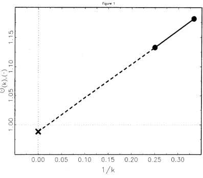
_u6_/24)}.

Figure 1 illustrates the nature of the extrapolation involved. For this figure a pseudo-random,

standard normal sample of size 4, {Xl = -0.20544, X2 = 0.33879, X3 = 1.39088, X4 = -1.02414},

was generated subject to certain constraints explained in Section 3.2. For these data J1.

=

0 and

thus 8 = 1. Plotted are the points

(8

(k),(.jl

l/k)

for

k

= 3 (the average of the 4 leave-l-out

estimates), k

=

4 (the maximum likelihood estimate), and k

=

00 (the jackknife estimate). It is

evident that the jackknife estimate is a simple linear extrapolation (the dashed line) of the line

determined by the maximum likelihood estimate and the average of the leave-I-out estimates on an

inverse sample size scale. Since 8 = 1, Figure 1 illustrates both the positive bias of the maximum

likelihood estimator and the negative bias of the jackknife estimator. Our Figure 1 is similar to a

figure in Efron (1982, Ch. 2, p. 7).

3. SIMULATION EXTRAPOLATION

3.1. Simulation Extrapolation Estimation

SIMEX estimation is a computational and graphical method-of-moments-like inference procedure

for assessing and reducing measurement error-induced bias. The method starts with the observed

data and the so-called naive estimator, i.e., the estimator computed from the observed data without

pseudo-random measurement errors to the data in a resampling-like stage and recalculating the naive

estimator again from the contaminated data. These estimators are used to establish a trend of

measurement error-induced bias versus the variance of the added measurement error. This trend is

then extrapolated back to the case of no measurement error, producing estimators with less bias,

and in some cases no bias, at least asymptotically. Details of the method and example applications

are presented in Cook and Stefanski (1992).

We adopt notation consistent with Cook and Stefanski (1992). We use U to denote the true

variate subject to measurement error (U is for unobserved), X to denote the measurement of U,

and Y and V to denote response and covariable variates respectively, should the latter be present

in the data. We assume initially that Xj

=

Uj

+

(JZj, j

=

1, ... ,n, where {Uj}f is a sequence

of unknown constants and {Zj}f is a sequence of independent standard normal random variables,

i.e., a functional measurement error model with additive independent normal error.

The estimator that would be calculated in the absence of measurement error IS denoted

8TRUE = T ( {Yj , Vj , Uj}n, where T represents the function applied to the data, e.g., for linear

regression T would commonly represent least-squares estimation. The so-called naive estimator,

i.e., the estimator calculated if measurement error is ignored, is obtained by replacing Uj with Xj

above, and is denoted 8NAIVE = T({Yj,Vj,Xj}f).

The pseudo data constructed by adding random errors to{Xj}} are denoted

j=l, ...

,n,

b=l, ... ,B,

where the added pseudo errors, {{Zb,j

Yi=df=l

are mutually independent, independent of the data

{Yj , Vj,Xj}I, and identically distributed, standard normal random variables.

The pseudo data are used to calculate

which in turn are used to estimate, by averaging,

b=l, ... ,B, (3.1)

(3.2)

The expectation in (3.2) is with respect to the distribution of {Zb,j

}j=1

only.

Note that 8(0) =

8

b(0) = 8NAIVE' Although analytic determination of 8(A) for A

>

0 is

sometimes possible, it can always be estimated with arbitrarily small variance by generating a

estimator

th(A)

for each b= 1, ... ,B, and estimating

O(A)

by the sample mean of

{Ob(A)}f.

This

is the simulation component of SIMEX.

The extrapolation step of SIMEX entails modelling

O(

A) as a function of A for A ~ 0 and extrapolating the model back to A

=

-1. This results in the simulation-extrapolation estimator

denoted 8SIMEX. The procedure is illustrated in the next section.

3.2. Estimating 0= exp(J.L) via Simulation Extrapolation

SIMEX estimation applies to the problem studied in Section 2under the interpretation that Xj

is a measurement ofJ.L with measurement error variance (12. Adding additional measurement error

with variance A(12 to

X}, ... , X

n , results in the estimator

8b(A)

= exp(X

+

(1

V):

Zb)

where

(1y).Zb

is the mean of the added pseudo errors. Doing this for b= 1, ... ,B, averaging the estimators, and letting B -+ 00 conceptually, results in

B

8(A) = lim B1

~

exp(X

+

(1

V):

Zb)

=

E{8b(A)

I

X} = exp(X

+

A(12/(2n)),

B-+oo ~

b=l

where the limit is justified by an appeal to the Strong Law of Large Numbers, and the expectation

can be found using moment generating function-like identities.

The functional form of

O(

A) is known in this example only because the required expectations can

be obtained analytically. The measurement error analyst will always have available

((O(A),

A) :

A

>

O}, but will seldom know its functional form. Thus for this example we proceed under the

contrived assumption of ignorance of the functional form of 8( A).

SIMEX next calls for plotting 8(A) versus A for A

>

0, fitting a model to this curve and

extrapolating the curve back to A= -1, thereby obtaining 8SIMEX. Upon examining the plot of

B(A) versus A or by looking at residuals from the fit of a linear model, most data analysts would

arrive at the realization that log(iJ(A)) is exactlylinear in Aand hence determine the exact functional

form. Thus for this example SIMEX results in the estimator iJSIMEX = iJ(-1) = exp(X_(12

/(2n)).

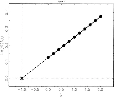
Figure 2 contains a plot of In(B('x)) versus A for 0

:S

,X

:S

2 (solid line), and the extrapolation

to ,X

=

-1 (dashed line), for the four-point data set set used in Section 2. The plotted points are for an equally-spaced grid of eleven ,X values spanning [0,

2],

and In(8SIMEX) at A

=

-l.

There is nothing special about the number or range of A values employed in this example, except

that both are large enough to provide convincing evidence of linearity. It transpires that for these

data BS1MEX = 1, i.e., exactly equal to O. Thus Figure 2illustrates both the positive bias of the maximum likelihood estimate, iJ(O), and the apparent unbiasedness of the SIMEX estimator.

that both

°

(n),(.) and

°

(n-l)'(-j, equal their expectations. Thus Figures 1 and 2 depict exact

expectedbehaviour of the maximum likelihood, jackknife and SIMEX estimators.

Indeed, a simple calculation shows that 0SIMEX is an unbiased estimator of 8 in this problem.

In fact, for what it's worth, 0SIMEX is the uniform minimum variance unbiased estimator of 8.

This is not a coincidence. If the naive estimator is a function of a sufficient statistic, then so too

will be the SIMEX estimator. Ifthe latter is unbiased, then it is necessarily uniform minimum

variance unbiased.

Lest we be accused of painting too rosey a picture of SIMEX with this example, we emphasize

that the unbiasedness of 0SIMEX depends crucially on knowing (72, being able to determine the

functional form of 9(A) exactly, and normality of the data. For simple problems O(A) often has

a simple functional form, and a little exploratory data analysis will often reveal it. However, the

strength of SIMEX does not depend on knowing the functional form of O(A). Our experience

indicates that even for complicated problems9(A) is well approximated by one or more of a handful

of simple functional forms (see Cook and Stefanski (1992) and Section 4 of this paper), and that

the approximations are generally more than adequate for applied work.

However, in most applications (72 is not known, and an estimate is used in its place. The

effect of this can be analyzed in the simple example described above. When (72 is replaced by s~,

0SIMEX = exp(X - s~j(2n )). Routine calculations involving normal and chi-squared moment generating functions show that this estimator has expectation anexp(J.l) where

2 [ 2 ](1-n)/2

an = exp((7 j(2n)) 1

+

(7 j{n(n - I)} .

A little analysis shows that an

2:

1 for all n and that n3

(an - 1) -+ (74j4 as n-+ 00. In other words

the SIMEX bias,

E(OSIMEX) -

8, is positive and of order n-3 for the case when (72 is estimated

by s~.

With regards to normality, SIMEX has no particular advantages or disadvantages relative to

other nonlinear estimators. Many non quadratic estimators that are unbiased under an assumption

of normality, fail to remain unbiased under non normality in general. In the particular example of

this section, it should be noted that normality of the data is important only to the extent that

it guarantees the independence of

X

and s~X", and that expectations of certain functions of these statistics are the same as those obtained from the appropriate normal and chi-squared distributions.

4. EXTRAPOLANT CHARACTERISTICS AND EDA

4.1 Exploratory Data Analysis and Quadratic Extrapolants

estimates, 9(oX), oX

>

O. The curves are necessarily smooth ifB is large enough and in some cases

have simple functional forms that are easily identified using exploratory data analysis techniques.

However, in most problems the curves will not have simple functional forms although there will

usually be some simple form that fits well. Th~ problem is finding it. Since not all exploratory

data analysts are created equal, it is difficult to present an objective description of a procedure

that relies on an exploratory modelling step.

In the simulations and examples that follow we fit simple quadratic extrapolants in each case.

Thus we avoid the problem of biasing the reported results by having prior knowledge of the

appropriate, or best extrapolant function. In doing so, we provide a lower bound on the performance

of SIMEX in the sense that statisticians are more competent curve fitters than our straw analyst

who fits only quadratic functions. However, it will be evident that our straw analyst does quite

well. The reason is that for many problems extrapolant curvature is slight and is well modeled by

a quadratic.

4.2 The Range ofoX

The simulation step can generate 9( oX) for all oX

>

O. There remains the problem of choosing a

range ofoX, say [0, AJ, over which to fit the extrapolant model.

Having developed SIMEX as an exploratory method for analyzing and describing the effects of

measurement error, we were led to consider initially A= 2. The plot of9(oX) for 0 ::; oX ::; 2, yields

immediate responses to queries about the effect of measurement error at levels two (oX = 1) and three (A

=

2) times as large as the nominal level (72 (oX

=

0). Note that if the naive estimate is

derived from measurements that are the means of replicate or triplicate measurements, then such

queries translate directly into questions about the adequacy of a single measurement.

Subsequent simulation studies designed to investigate the choice of A have been generally

inconclusive. This is good, since it suggests that SIMEX is relatively robust to choice of A. In

addition, some useful conclusions are possible for the problem of estimating regression coefficients

in large samples, under the assumption that B is large enough to ignore simulation variation.

Our observations are based on experience estimating regression parameters, suggesting that

extrapolant functions are often monotone, concave or convex, and have decreasing curvature as

A increases. In such cases if a quadratic extrapolant is employed, then there is a tendency to

undercorrect for the effects of measurement error. The reason is that the constant-curvature

quadratic will diverge from the increasing-curvature true extrapolant as A -+ -1. The larger

the value of A, the greater the undercorrection. However, a little undercorrection is desirable if

associated with the choice of A when quadratic extrapolants are fit.

5. SIMEX COMPLEMENTS TO JACKKNIFE THEORY 5.1 The Jackknife in SIMEX Clothing

The connection between SIMEX and the jackknife suggests an alternative formulation of the

latter. Let {) (n-j),(-) denote the average of thenCjleave-j-out estimators8(n-j),(k)' k

=

1, ... , nCj,

based on samples of size n - j. For some fixed positive integer jmax ::; n - 1 and for Aj = j /(n - j), j = 0,1, ...,jmax, (0 ::; Aj ::; A= jmax/( n - jmax)), calculate

9(

Aj) =

8

(n/(Aj+l»,(.) •

Next plot 8(Aj) versus Aj, examine this plot, and fit a model extrapolating the curve to A

=

-1.

The extrapolant at A= -1 is the modified, reduced-bias jackknife estimate.

The mapping between Aj and j (the number of points left out) is best understood in the context of estimating ()

=

f(p.) via f(X) with normally distributed, N(p.,u2), data. In this case X(n-j),(k)

and X

+

UAZb are identically distributed when Aj

=

j/(n - j). It follows that f(X(n-j),(k») and f(X

+

UAZb) are identically distributed and thus possess the same moments, inparticular

the same bias and variance. This is the key property relating SIMEX to the jackknife. Note that

j

= -

00 corresponds to Aj

=

-1; this correspondence is part of the explanation for our definition

of jackknife estimator as a leave-(-00)-out estimator.

Others have studied the use of higher-order jackknife modifications (Gray et

at.,

1972, 1975;

Schucany et

at.,

1971). Thus there is little new here except the proposal to examine the plot of

O(

A) versus A and use exploratory methods to suggest an appropriate extrapolant function.

The idea is intriguing. The usual two-point jackknife is a function of only two summary statistics,

-

-O(n),(.), and 8(n-l),(-). Thus there is an inherent loss of information relative to the proposed

modification which is a function ofn summary statistics when A= n - 1.

Despite this advantage of the proposal, we doubt that it will supplant the usual jackknife. The reasons are twofold. First there is the inescapable bias-variance compromise. Reducing

bias increases variability and thus there is always a point beyond which further bias reduction

is counterproductive. For many real problems the usual jackknife seems to be near this optimal

point. Second is the matter of knowing how to use the additional information in the modified

proced ure. The discussion in Section 4 makes clear that knowing

8(

A) for large A is useful only if the exact extrapolant function is known. When an approximate extrapolant is employed attention

should be focused on A in a neighborhood of O. Applying the rule-of-thumb region, 0 ::; A ::; 2,

sugested by our experience with SIMEX to the proposed modified jackknife bounds j via the

inequality 22 Aj

=

j /(n - j), i.e., j ::; 2n/3.

•

simulation employed the model of Section 3.2 with n = 5. Seven estimators were studied: the

maximum likelihood estimate (MLE); the two-point linear jackknife estimator (LJ); three-, four-,

and five-point quadratic modified jackknife estimators, i.e., the modification suggested above using

a quadratic extrapolant (QJ3-QJ5); the SIMEX estimator with s~ in place of u2 _{(SIMEX1); and}

the SIMEX estimator with known u2 (SIMEX2). One-hundred thousand data sets were generated and analyzed.

The bias-corrected estimators do a good job of eliminating bias. Reductions ranged from 94% for

LJ, to 100% for SIMEX2. All of the pairwise t-tests comparing MSEs are statistically significant,

except the test comparing QJ3 and SIMEXl. However, except for SIMEX2, there is little practical

difference between the estimators.

Of the three quadratic-extrapolant estimators the worst performing was QJ5 corresponding to

A= 4 which is much greater than the rule-of-thumb cutoff of 2. In contrast QJ3 and QJ4, with

A= 2/3 and 3/2 respectively, performed better.

5.2 Jackknifing a Sample of Size One

In this section we use the term jackknife to denote both the specific techniques associated with

the name, and the broader notion of a generally useful tool for reducing bias.

The connection between SIMEX and the jackknife makes clear that the essential role played

by multiple observations in the latter is to provide a measure of variability. Jackknifing should

be possible, in principle, with a sample of size one provided an external estimate of variability is

available. One such manifestation of the jackknife under these conditions is SIMEX estimation.

The example in Section 3.2 makes this clear. Reexamination shows that, given either the raw

data

{X

j}l,or

X

and either knowledge of u 2 or an independent estimate of it, say &2, it is possible to construct the SIMEX estimator. In the case that only

X

is given, the simulation step of SIMEX differs only in that the pseudo errors are generated from a N(O, &2/n ) distribution and added to

X,

where &2 is either the known or estimated value ofu2•

Thus we now consider bias reduction in the estimator 0NAIVE = f(X) of f(J.L), assuming that

X is normally distributed with mean J.L and known variance u2_{• We know how SIMEX is to be}

applied. Simulation is used to estimate O(A) = E{f(X

+

U..;'>:Zb)

I

X} for 0 ~ A ~ 2, the plot

ofO(A) vs Ais examined, and a model is fit to the curve. Extrapolation of the model to A = -1

results in the reduced-bias SIMEX estimator.

Note that for the simple models studied in this section, O(A) can be calculated by numerical

integration more easily and efficiently than by simulation. However, the simple models are studied

..

numerical integration is not feasible and thus we maintain the simulation component.

We now show that if the true extrapolant is employed, then for a general class of functions

f,

the SIMEX estimator is unbiased. The results that follow hold for smooth functions

f,

although the smoothness requirements are much greater than the common regularity conditions (one or two

continuous derivatives) usually encountered in mathematical statistics. A minimum requirement is

that

f

be analytic, i.e.,has a convergent power series expansion, and furthermore that expectation and summation can be interchanged in the power series expansion of

f.

The necessary smoothness conditions have been studied elsewhere (Stefanski, 1989) and will not be examined here. In the

following i =

yCl.

LEMMA 1. IfZ1 and Z2 are independent and identically distributed standard normal variates, then E{(Zl+iZ2)n} =0, n=1,2, ....

PROOF. The result can be verified by binomial expansion and direct calculation. Alternatively,

consider that Zl+~Z2 has a N(O, l+A)distribution and thus E{(Zl+~Z2)n}is proportional to (1

+

A)n/2. Let A-+ -1 to establish the result. This proof actually uses the result of Lemma 2,

although in an easily justified case.

_••

LEMMA 2. If f is sufficiently smooth and Zl and Z2 are independent and identically distributed standard normal variates, then

(5.1)

PROOF. Under the assumptions on

f,

and upon appeal to Lemma 1,

00 f(n)(p)crn

>'~~1

E{I(p

+

crZ1

+

Vf"

crZ2)} =

>'~~1

E{I(p)

+

L

n! (Zl

+

Vf"

Z 2)n} n=l

00 f(n)(p)crn

=

E{I(p)

+

L

,

(Zl

+

iZ2)n}

n.

n=l

00 f(n)( ) n

= f(p)

+

L

~

cr E{(Z1

+

iZ2

t}

= f(p), (5.2) n.

n=l

completing the proof. ••

Henceforth, we define a sufficiently smooth function

f

to be one for which the result of Lemma 2 holds.

The exact SIMEX extrapolant is just

tip)

=

E{I( X

+

..;>:

cr Zb)

I

X}

and the corresponding

the latter equality following from Lemma 2. That is, the exact SIMEX estimator is unbiased.

Lemma 2 and the unbiasedness of the exact SIMEX estimator have an interesting (and amusing)

intuitive explanation. Estimator bias generally results from the fact that for a nonlinear function,

g, and random variate X, E {g( X)} =Fg( E {X}) in general. In fact the latter is true in general only ifX is degenerate, i.e., Var(X)=O, in which case E{xn} = (E{X}t for all n.

In the following we define Var{W} = E{W2} - (E{W})2 for complex-valued random variables

W. Also if WI and W2are two complex~valued random variables we define their covariance as

Cov{WI ,W2} = E{WI W2} - E{WdE{Wd. It will become evident that this is a useful departure

from convention. The reader is warned that these definitions give rise to some unusual looking

results.

It follows from Lemma 2 that the complex variate W = J.l

+

(1ZI

+

i(1Z2, where ZI and Z2

are independent standard normal variates, has mean E{W} = J.l, and variance Var{W} = O. In

fact Lemma 2 shows that E{wn} = J.ln = (E{w})n for all n ~ 1. Thus W behaves very much

like a degenerate N(J.l, 0) random variate with respect to expectation, in the sense that for any

smooth g, E {g(W)} = g( E{W}). Since adding i(1Z2 to (1ZI annihilates (1ZI in an expected value

sense, we refer to i(1Z2 as the anti-measurement error of (1ZI. We now have the amusing, yet

fairly descriptive paraphrasing of Lemma 2, "measurement error-induced bias is annihilated by the

addition of anti-measurement error."

A simple example illustrates these ideas. Consider the problem of estimating f(J.l) = J.l2. The

estimatorf(X) = X 2is biased because of the measurement error X -J.l = (1Z. Let X* = X +i(1Zb.

A candidate estimator is X; = X2 - (12Z;

+

2iX(1Zb. This has expectation E{ X;} = J.l2 and is

thus unbiased. We have annihilated the measurement error in an expected value sense. However,

the new estimator has certain deficiencies, namely it is a complex variate and it depends on the

arbitrary, generated pseudo error, Zb. These deficiencies are remedied by taking the real part of

the estimator, and then taking expectations conditional on X; or simply by taking expectations

conditional on X, since the imaginary part vanishes upon conditional expectation. We are left with

the unbiased estimator 0SIMEX = X2- (12.

Although the previous paragraph dealt with f(J.l) = J.l2 the main points apply to any smooth

function f: a) E{f(X

+

i(1Zb)} = f(J.l); b) the imaginary part off(X

+

i(1Zb) has zero conditional

(on X) mean; and c) E{f(X

+

i(1Zb)

I

X} is an unbiased estimator off(J.l).

5.3 Variance Estimation

The jackkknife is used at least as often for variance estimation as it is for bias reduction (Tukey,

1958; Efron, 1982). We now examine SIMEX in regards to variance estimation.

The basic building blocks of a jackknife variance estimate are the n differences

~k

= O(n-I),(k) -

0

(n-I),(.)' k = 1, ...

,n.

The jackknife estimate of variance is n-I(n - 1)~~=I ~l.

In the SIMEX version of the jackknife with sample size = 1, corresponding quantities are

). >

O.

We use the problem of estimating exp(ll) to illustrate the manner in which these differences

are employed in variance estimation. The SIMEX estimator is 0SIMEX

=

exp(X - (72/2). It has expectation exp(ll) and its variance is easily calculated and shown to be {exp((72) - I}exp(21l).

For this problem,

The variance of this difference is easily calculated and found to be,

Note that since O()') = E{Ob().)

I

X},

Var{~().)}= E{Var{~().)

I

X}}

= E{Var{~().)

I

X, O().)}}.

(5.3)

The variance of 0SIMEX' which we have already calculated directly, can also be obtained by

taking the limit as). ---+ -1 ofVar{~().)},viz.,

Var{OSIMEX} = - lim Var{~(>.)}.

A-+-I (5.4)

It is easily verified that taking the indicated limit results in the correct variance. The formula is also easily checked for the case !(Il) = 1l2

• Note that ~(O)= 0and thus Var{~(O)}= O. Since for

>.

>

0, Var{~(>.)}

>

0, it is to be expected that as this curve is extrapolated to ).

<

0, Var{~().)} takes on negative values. This seemingly preposterous result is due to our definition of variance for

complex-valued random variates, e.g., Var{i(7Zb}

=

_(72. Since

Os

1MEX is itself a limit as>. ---+ -1,

the previous formula is naturally expressed as

Var { lim

O().)}

= - lim

Var{~(>.)}.

Before demonstrating the correctness of the formula in general we describe its relevance in practice.

Inproblems that defy analytic treatment, the variance of the SIMEX estimator can be estimated

by: 1) calculating S~(A), the sample variance of the (h(A), b

=

1, ... ,B, for each A, thereby

obtaining an unbiased estimator of Var{6.(A)

I

X}, which by (5.3) is also unbiased for Var{6.(A)};

2) plotting s~(A) versus A; and 3) modelling the curve and extrapolating back to A= -1. The

result is an estimator, albeit an approximate one when an approximate extrapolant is used, of

-Var{8S IMEX}·

LEMMA 3. If

f

is sufficiently smooth, then (5.5) holds.

PROOF. The derivation of the variance formula depends on a simple but subtle point that is best attended to initially. Lemma 2 shows that when f is smooth, 8b(A) = f(X

+

';>:(7Zb) has

expectation E{(h(A)} -+ f(J.l) as A-+ -1. When f is smooth

P

is also smooth, and thus Lemma

2 also shows that E{8~(A)} -+ f2 (J.l) as A-+ -1. It follows that

(5.6)

Now since 8(A) = E{Ob(A)

I

X}, it follows that Cov{fh(A), 8(A)} = Var{8(A)}. Thus, via the usual variance decomposition,

Var{8b(A) - 8(A)} = Var{8b(A)}

+

Var{8(A)} - _{2Cov{8b(A), 8(A)}}

=

Var{8b(A)} - Var{8(A)}.

In light of (5.6) it is seen that

lim Var{8b(A) - 8(A)}

= -

lim Var{8(A)}

=

-Var{8(-1)}

=

-Var{8SIMEX}'

,\--1 ),-+-1

completing the proof.

_••

SIMEX is now a complete package for the problem of estimating f(J.l) from X '" N(J.l, (72)

with (72 known or independently estimated, say be &2. Pseudo errors are generated to obtain

8b(A)

=

f(X

+

&';>:Zb), b

=

1, ... ,B. The sample mean, 8(A), and variance, S~(A),of_{8b(A)}f

are then calculated for several A. These are plotted as functions of A, modelled and extrapolated

back to A= -1. The extrapolated mean function yields the estimator 8SIMEX; the extrapolated

variance function, multiplied by -1, yields an estimator of Var{ 8SIMEX}. The method is exact,

in the sense of producing unbiased estimators, when (72 is known, i.e., &2 = (72, and the exact

For the problem of estimating J(Jl) = exp(Jl), it is readily verified that as B -+ 00,

81

(A) -+

V(X,A), where V(X,A)

=

Var{th(A)

I

X}

=

{exp(2(12 A) - exp((12 A)}exp(2X) is the exact

extrapolant function for variance estimation. Thus if the exact extrapolant is employed, the

SIMEX estimator of Var{OSIMEX} is -v(X,-1). Under the assumed normality, -v(X,-1) is

the uniform minimum variance unbiased estimator ofVar{OSIMEX}' It is tempting to debunk this optimality in light of the small likelihood of identifying the exact variance extrapolant function in

this case without prior knowledge its the functional form. However, the important point is that

the approximate SIMEX variance estimator, approximates an estimator that makes efficient use of

the data.

Cook and Stefanski (1992) suggested the use of pseudo errors contstrained to have certain

population moments, as a means of reducing variability in the Monte Carlo estimate of 8(A) and

decreasing computation time. However, they did not consider SIMEX variance estimation. In

order for the variance estimator suggested herein to be valid in general, the pseudo errors must be

independent and identically distributed.

5.3.1 Variance Estimation Simulation

We now illustrate this procedure with an example and study its performance via simulation. We

take f(Jl) = Jl/(1

+

exp(-Jl)). This function is not analytic and thus Lemma 2 does not apply. We

chose this function for two reasons. First, to demonstrate the utility of the method even when the

mathematical theory does not apply and an approximate extrapolant, a quadratic, is necessarily

employed.

Second, is the relevance of this function to understanding measurement error in logistic

regres-sion. The normal equations for simple logistic regression are L:j=dYj - G(o:

+

,BUj)}(l, Ujf = (0, O)T where G is the logistic distribution function. IfUj is replaced by a measurement _{X h} then the normal equations lose the essential feature of Fisher consistency since

E {{Yj - G(o:

+

,BXj)}(I, Xj?} =G(o:

+

,BUj)(I, Uj)T_

E {G(o:

+

,BXj)(I, Xj?}

:f:

(0, O?

Nonlinearity of the functions G(t) and tG(t) is responsible for the lack of Fisher consistency. The

latter is just the function f(t) = t/(1

+

exp(-t)) chosen for our simulation.

For the simulation study Jl = 1 was fixed. The measurement error variance (12 had levels

0.25, 0.50, 0.75 and 1.00. Two independent N(Jl, 2(12) measurements ofJl were generated as well

as a second independent sample of size d

+

1 of N(Jl, (12) measurements. The first sample of size

construct an estimate of(72 based on d degrees of freedom. This was done for d= 1, 16, 256 and

00, i.e., (72 known.

This design allowed us to control both the measurement error variance and the precision of the

independent estimate, 172_{, of(72 required by SIMEX, while also allowing for the calculation of the}

standard, linear-extrapolated jackknife estimator from the initial sample of two measurements.

The study compared three estimatorjvariance estimator pairs: the maximum likelihood

estima-tor 0NAIVE = f(X), with ~-method variance estimator {f'(X)p 172; the SIMEX estimator and

corresponding variance estimator employing quadratic extrapolants for each; and the jackknife

es-timator and corresponding variance eses-timator based on the sample of size 2. The SIMEX eses-timator

was calculated with B

=

1000 and 4000. We report on only the results for B

=

4000. The smaller

value of B was studied as a check on the adequacy of B = 4000. The results for B = 1000 and

B = 4000 were similar. For each combination of(72 and d, 25,000 replications were performed.

The intent of the study is to show that even with the use of simple quadratic extrapolants, and

for a case where the exact theory does not hold, and when(72 is replaced by172,that SIMEX reduces

bias as well as the jackknife, and that the proposed variance estimation method is comparable to the

jackknife variance estimator as an estimator of the variance of the reduced-bias jackknife estimator.

Relevant results of the study are displayed in in Figures 3a-3d and 4a-4d.

With 25,000 replications, visually detect ably differences and statistically significant differences

are roughly the same. In order to preserve clarity in the figures we elected not to display standard

errors. However, some feeling for the simulation variability can be inferred from the plots upon

realizing that the jackknife procedure made no use of the data used to generate the independent

estimate of(72. Thus the four dashed lines in Figures 3a-3d and in Figures 4a-4d are independent

replicates.

Figures 3a-3d contain plots of relative bias as functions of(72 for each d. The SIMEX estimator

displayed uniformly smallest bias across levels of(72 and d, with the jackknife a close second.

Figures 4a-4d display plots of the (mean of the variance estimator)j(true estimator variance)

as functions of(72 for each d. In all cases the SIMEX procedure came closest to the ideal value of

unity, i.e., unbiased variance estimation. The true variances of the SIMEX and jackknife estimators

were virtually identical over all factor level combinations in the experiment. Thus the differences

in Figures 4a-4d are due almost exclusively to differences in the means of the estimated variances.

Both procedures underestimate variability, the jackknife more than SIMEX.

These results are not in conflict with the well-known conservativeness of the jackknife variance

estimator as an estimator of the variance of the initial estimator, the maximum likelihood estimator

in this case, and not as an estimator of the variance of the reduced-bias jackknife estimator.

Figures 5a and 5b display an example of the quadratic mean and variance extrapolations used

in the SIMEX procedure. Figures 5a and 5b were constructed from a data set generated as in

the simulation with cr2 = 0.5 and d = 256, and employed B=1000 replications in the simulation

step. The unusually poor fit of the extrapolant in Figure 5a suggested that B was not large

enough for this particular sample, i.e., an unusually variable sequence of pseudo errors had been

generated. We reanalyzed the data set taking B = 16,000 resulting in the quadratic mean and

variance extrapolants plotted in Figures 5c and 5d. Comparison between Figures 5a and 5c suggests

that even though our simulations failed to reveal noteworthy differences between B = 1000 and

B

=

4000, that differences might be detected at even larger values ofB.

5.3.2. Jackknife Variance Estimation Revisited

The SIMEX description of the jackknife presented in Section 5.1 and Lemma 3 suggest an

alternative method of deriving a jackknife variance estimator. Suppose that A

=

l/(n - 1) so

that the usual linear jackknife is obtained. Lemma 3 then suggests fitting a line to the two points

(Aj, Vj), j = 1,2 where Al = 0 and VI = 0, and A2 = l/(n - 1) and V2 = n-1 L~ ~~, the population variance of the n differences ~k = (}(n-l),(k) - (} (n-l),(.); then extrapolating the line

back to A = -1, resulting in - V2/ A2. Upon multiplication by -1 we arrive at the new variance

estimator, n-1(n - 1)L~=l ~L that is, the usual jackknife variance estimator. In other words, the

ususal jackknife variance estimator is an extrapolation of the form (5.5), but with an approximate

(linear) extrapolant.

Itmay appear that this result was fudged by use ofthe divisornin the definition ofV_{2 •} However, for SIMEX variance estimation, S~(A)is an unbiased estimator of the variance of

8

b(A) about its

conditional mean (}(A). Likewise V2 should be an unbiased estimator of the variance of8(n-l),(k)

about (} (n-l),(-)' In the special case that

iJ

is the sample mean, then either exactly for finite

samples and normally distributed data, or approximately for large samples upon appeal to the

Central Limit Theorem, the conditional distribution of8(n-l),(k) given (} (n-l),(.) is normal with

mean

8

(n-l),( .). Itfollows that the divisor n in V₂ yields an unbiased estimator of the appropriate

conditional variance. The same argument applys asymptotically for non-sample mean statistics

after linearization.

6. JACKKNIFE COMPLEMENTS TO SIMEX THEORY

In this section we extend the jackknife-like variance estimation procedure for SIMEX estimators

Cook and Stefanski (1992).

In Section' 3.1 we introduced the function T to denote the estimator under study. We now

introduce a second function, TYar to denote an associated variance estimator. That is, with

6TRUE = T( {Yj, Vj, Uj}f), TYar({Yj,ltj,_{Uj}f) is an estimator of Yar{6TRUE}' We allow} T to be p-dimensional, in which case TYar is pXp-matrix valued, and variance refers to the

variance-covariance matrix. We use r2 _{to denote the parameter Yar{6TRUE}' TTRUE to denote the}

estimator TYar({Yj, Vj,Uj}f), f&AIYE to denote the naive estimator TVar({Yj, Vj,Xj}f), and

so on.

6.1 Multivariate Anti-Measurement Error

We start this section with a generalization of Lemma 2 to multivariate normal random variates.

LEM MA 4. If

f

is a sufficiently smooth function from RP to Rq, P, E RP, and Zl and Z2 are independent and identically distributed p-dimensional N(O, n) random vectors, then

(6.1)

PROOF. The assumed smoothness allows us to represent the qcomponents of

f

as multivariate

power series and to exchange expectation and series summation. First assume that

n

is the identity

matrix. In this case the key step in the proof entails showing that

when at least one of the nonnegative interger powers Tj

>

0, where Zl,j and Z2,j, j

=

1, ...,pare

the components of Zl and Z2 respectively. The truth of this assertion follows from independence

and appeal to Lemma 1. It then follows that upon taking expectations in the series expansion of

f(p,

+

Zl

+

iZ2)around p" that all terms vanish except the first, that is f(p,).

For the case with general

n

define9 viag(t)

=

f(p,

+

n

1 / 2t) where

n

1_/2_{is the symmetric square}

root of

n.

By the independence case just established, E{g(n-1_/2Zl

+

in-

1_/2_Z2)}

₌

_{g(O). Invoking}

the relationship between

f

and 9 establishes the result.

_••

6.2 Exact SIMEX, Finite-Sample Theory

In this section we assume that 6TRUE = T( {Yj ,ltj,Uj}f) is an unbiased estimator of(Jand that

TYar({Yj 'Vj,Uj}l) is an unbiased estimator of Yar{6TRUE}' Furthermore we assume that both

T and TYar are smooth functions of the arguments Uh . . . ,Un'

that

lim E{8(An = E{8(-In = 8,

A-+-l

and

Further appeal to smoothness, Lemma 4, and upon invoking our definition of variance in the

case of complex-valued p-dimensional variates, show that

Var{OSIMEX}

=

Var{O(-In

=

lim Var{O(An

A-+-l

=

lim Var{Ob(An - lim Var{Ob(A) - O(A)}

A-+-l A-+-l

= Var{8b(-In - lim Var{Ob(A) - O(An. (6.2)

A-+-l

But the fact that TTT is smooth whenever T is smooth, and further appeal to Lemma 4 show

that

A A AT A A T

Var{8b(-In = _{E{8b(-I)8b (-In - E{8b(-I)}(E{8b(-In)}

A AT T

= _{E{E{8b( -I)8b (-1)}

I

{Yj, Vj,Xj}fn - 88

A AT T

= _{E{8TRUE8TRUE} - 88}

= Var{OTRUE}

SIMEX estimation can be used to estimate (the components of) r2• That is, f;

(A)

=

TVar({Yj 'Vj,Xb,jpnf) is calculated for b = I, ... ,B, and upon averaging and letting B -- 00,

results in f 2(A), and so on. Furthermore, the sample variance matrix of {ih(Anr=l' call it

S1(A),

is

an unbiased estimator ofVar{8b(A)-O(A)

I

{Yj , Vj,Xj}f} for all B

>

1 and converges in probability

to its expectation as B -- 00. It follows that E{si(An = Var{Ob(A) - O(An.

The plots of (the components of)

si

(A) versus A

>

0, extrapolated back to A= -1 provide an estimator of

The estimator is unbiased if the exact extrapolant is used. In light of (6.2) the difference,

f§IMEX - si( -1), is an unbiased estimator of Var{OSIMEX}'

SIMEX estimation is now a complete package for the special case of this section. The simulation

unbiased estimator of 8, and extrapolation of (the components of) the difference, f2(A) - Si(A) to

A

= -1 provides an unbiased estimator of Var{OSIMEX}'

6.2.1. Components-of-Variance Estimation

The components-of-variance problem provides a simple yet informative illustration of these ideas.

Suppose that U1, ... , Un are independent and identically distributed N({lu, 8). Thus 0TRUE

=

sh

and 0NAIVE

=

s~. Cook and Stefanski (1992) show that for this problem O(A)

=

s~

+

A0'2 and

thus 0SIMEX = s~_0'2. The normality ofU1, ... , Un is significant only to the extent that it allows

us to easily identify an unbiased variance estimator, ftRUE' of 0TRUE'

Itis readily verified that r 2

=

282/(n - 1), ftRUE

=

2st/(n

+

1),

A2( ') _ _2_ {( 2 '2)2 2A20'4

+

4A0'2s~}

r A - Sx

+

AO'

+

1 '

n+1

n-and

2 (A) _ 2A20'4

+

40'2AS~

sa - n - 1 .

The difference, f2(A) - Si(A)

=

2si/(n

+

1), is constant in Aand thus extrapolation to A

=

-1

is trivial. It is equally trivial to show that the constant difference, 2s1 / (n

+

1), is an unbiased

estimator of Var{OSIMEX}'

6.3 Exact SIMEX, Large-Sample Theory

In many problems, even in the absence of measurement error, the functions T and TVar do not

yield unbiased estimators, but do so only asymptotically, i.e., they yield consistent estimators as

the sample size, n -'> 00. We now argue heuristically that the SIMEX variance estimator works

asymptotically in general for such problems.

Our intent is explain how SIMEX works in large samples and not to provide rigorous conditions

under which the asymptotic results are valid. These are best handled on a case-by-case basis. We

begin the heuristics by replacing the finite sample estimators with their large sample linearizations,

that are assumed to exist.

Thus we let

_ 1 n

(}TRUE = (}

+ -

L

IC(Yj, Vj, Uj , (}),

n.

;=1

Related quantities required in SIMEX estimation are

. 1 n

theA) = 8(A)

+;;

LIC(Yj, Vj,Xb,j(A),8(A)), j=l

f;(A) =

:2

t

IC(Yj, Vj, Xb,j(A), 8(A))ICT(Yj , Vj, Xb,j(A), 8(A)), j=l

and

f2(,X) = :2

t

E{IC(Yj, Vj, X b,j(A),8(A))ICT(Yj, Vj ,Xb,j(A),8(A))

I

Yj , Vj,Xj}. j=l

Itis now a simple exercise to verify that all of the results from the previous section hold under the assumption that IC is a smooth function ofUj. Thus for SIMEX and SIMEX variation estimation

to work in large samples, smoothness of the functions T and T_{Var is not important} per se, but

rather it is smoothness of the influence curve that is relevant.

These large-sample heuristics are useful for they indicate the key components involved analyzing

SIMEX in large samples, namely linearization and smoothness of the linearized form, but they hide

the fact that a rigorous demonstration is quite involved. We illustrate this with a detailed analysis

of simple linear regression in the presence of measurement error.

6.3.1. SIMEX Variance Estimation in Simple Linear Regression

The regression model under investigation is Yj

=

Q

+

{3Uj

+

Ej, j

=

1, ... , n, where it is assumed

that the equation errors

{E

j}I are identically distributed with E{

Ed

=

0

and Var{

Ed

=

(1;,

mutually independent, and are independent of the measurement errors. Furthermore we assume

the functional version of this model,

i.e.,

that

Ul, ... , Un

are nonrandom constants. We add the

regularity condition that the sample variance of{Uj}I converges to

(1&

>

0, as n -- 00. This is

stronger than is necessary, but simplifies the presentation.

We will not address asymptotic normality per se, since this follows from the easily established

asymptotic equivalence of the SIMEX estimator and the much-studied method-of-moments

estima-tor (Fuller, 1987, pp 15-17); see also Lombard et

at.

(1993). Our focus is on variance estimation.

Define SyU

=

n-1L(Yj - Y)(Uj - (;) and Suu

=

n-1L(Uj - (;)2, etc. We proceed under the

minimal assumptions that: 1) Syy

=

{32(1fJ

+

(1;

+

op(l); 2) vn(SyX - Suu{3)

=

Op(l); and 3)

vn(Sxx - Suu - (n - 1)(12In)

=

Op(l). Note that 3) implies that Sxx

=

(1fJ

+

(12

+

op(l).

We consider estimating8= {3. Thus

• SYU

where O";,TRUE IS the

true-The estimator 0TRUE is unbiased in finite samples. However, the results of Section 6.2 do not

apply since the estimator is not a sufficiently smooth function of U1 , ••• ,Un' Indeed, if we view

0TRUE as a function of_U1alone, then it has the form g(Ud whereg(U1) = (dU1 +e )J(aui +bU1 +c)

for suitably defined real constants a, .. . , e. The quadratic in the denominator has either one real root or two complex roots, since Suu ~ O. In either case the function g(w) of the complex variable

w has at least one singularity in the complex plane and this violates the assumed smoothness (Stefanski, 1989).

D fi 2 2/( S ) d -2 (S )-1A2

e ne T = (1E n uu an TTRUE = n UU (1E,TRUE'

regression mean squared error. For this problem

(6.3)

where

A 1~ - I >

Nb(>') = :;; L)Yj - Y)(Xj

+

(1V

>.

Zb,j)

j=l

Db(>') =

~

t

{(Xj -

X)

+

(1v'>:(Zb,j - Zb)}2.

n . 1

J=

Define

N(>') = E{N_b(>.)

I

{Yj,Xj }} = SyX,

N(>')

=

E{Syx}

=

Suuf3,

- A

(n-l)

2

D(>.)

=

E{Db(>.)

I

{Yj,X j }}

=

Sxx

+

-n- >'(1,

(n-l)

2

(n-l)

2

D(>')

=

E{Sxx

+

-n- >,(1}

=

Suu

+

-n-

(>.

+

1)(1 .

The Cauchy-Schwartz inequality is used to show that

(6.4)

Conditioned on {Yj, X

j}l,

the right hand side of (6.4) is proportional to the reciprocal of a

noncentral Chi-squared random variable with n - 1 degrees of freedom and thus has its first k

Define

o

(A)

=

N(A) Nb(A) - N(A)Db(A)jD(A)

b D(A)

+

D(A) .

Then Ob(A)

=

Ob(A)

+

Rb(A) where

where

O(A)

=

N(A) N(A) - N(A)D(A)j D(A)

D(A)

+

D(A) .

In the Appendix it is shown that the remainder terms, Rb(A) and R(A), can be ignored

asymptotically. Thus upon employing the linearizations Ob(A) and O(A) it follows that

Si(A)

=

Var{(h(A) - O(A)

I

{Yj,Xj}n

~ Var{Ob(A) - O(A)

I

{Yj,Xj}r}

A0'2 { N 2 ( A ) 2 N(A)Sy x}

= nD2(A) Syy

+

D2(A) (4Sxx

+

2AO' ) - 4 D(A) .

For the linear regression model

and it is readily seen that

Of course nr2_{(A) also has the same limit asymptotically.}

Assuming that the exact extrapolant function is employed, the validity of SIMEX variance

estimator depends on

The indicated limit coincides with the asymptotic variance reported in Fuller(1987, pp 15-17).

The function, n{r';(A) - Si(A)}, that must be extrapolated to obtain the SIMEX variance

over a useful range of conditions. We will not provide evidence of this claim electing instead to

address this issue in a more complicated problem in the next section.

6.3.2. SIMEX Variance Estimation in Simple Logistic Regression

Logistic regression provides an example for which SIMEX theory is exact in neither finite samples

or asymptotically, yet has been shown by Cook and Stefanski (1992) to be competitive with

estimation methods that are optimal asymptotically. We now present an example demonstrating

the SIMEX variance estimator based on a quadratic extrapolant in a nontrivial application.

We make use of data from the Framingham Heart Study. The model we study relates Y =CHD,

an indicator of coronary heart disease over an eight-year period following enrollment, to systolic

blood pressure (SBP).

The data contain blood pressure measurements at two-year intervals during the study. We make

use of the first two such measurements and work under the assumption that on a logarithmic scale

these are replicate measurements; see Carroll and Stefanski (1993) for a discussion of the replicate

measurements assumption. Thus with Xl and _{X 2}denoting the logarithms of the two blood pressure

measurements, our working assumptions are that Xl = U

+

V2(1Z1 and X 2= U

+

V2(1Z2 where Zl and Z2 are independent measurement errors. Thus the best measurement, X = (Xl

+

_{X 2})/2,

has mean U and variance (12. Implied by our assumptions is the definition of U as the long-term

average In(SBP).

We have subsetted the data, selecting data on males only, and eliminating cases with missing

information. The resulting sample size is 1615. Since it is unlikely that data are missing at random,

we view our analysis as illustrative only.

A components-of-variance analysis results in the estimate 0-2 = 3.15X 10-3 corresponding to an

estimated linear model correction-for-attenuation (the inverse of the reliability ratio) of1.21.

Table 2 displays the results of three estimator/variance estimator combinations along with bootstrap variance estimates. The NAIVE procedure refers to ordinary logistic regression of Y

on X (= the average of the two measurements). Standard errors were obtained from the usual large-sample, inverse-information variance matrix estimate.

The SUFFICIENCY procedure refers to the method based on sufficient statistics as described

in Stefanski and Carroll (1985, 1987). This is a conditional likelihood-based procedure and is

known to be asymptotically optimal under certain conditions. Itprovides a benchmark with which to compare the SIMEX procedure. Standard errors were obtained as for the NAIVE procedure

employing the inverse, conditional-information matrix.

described in Section 6.2, with

T

and

TVAR

the usual,

i.e.,

non-measurement error, maximum

likelihood estimator and inverse information matrix respectively, and with B

=

1000.

In both the SUFFICIENCY and SIMEX procedures, the estimate

;,2

was employed as if it were

the known. This is not unreasonable in light of the sample size.

Five hundred bootstrap samples were drawn and analyzed for the purpose of obtaining bootstrap

standard errors for each of the three procedure.

Table 2 shows that the two measurement-error procedures result in nearly identical analyses

that differ predictably from the NAIVE procedure. The almost-constant differences between the

bootstrap standard errors and the procedure-based standard errors, and the relative magnitudes

of these differences suggest two conclusions. First is that the SIMEX standard error estimates are

comparably to the conditional likelihood-based estimates. Second is that all ofthe procedure-based

standard error estimates do an adequate job of estimating variability.

7. SUMMARY

The close relationship between SIMEX and the jackknife established in this paper adds much

credibility to the former. The SIMEX simulation step, corresponds to the jackknife leave-j-out

step, and the extrapolation steps in both procedures are conceptually identical.

In addition to providing· theoretical justification for SIMEX estimation, the investigation of

SIMEX as a variant of the jackknife made obvious the variance estimation procedure described in

Section 6. Except for the fact that the theory assumes (1"2 to be known, SIMEX provides a widely

applicable method for statistical inference in the presence of measurement error.

In situations where (1"2 is estimated and the estimation variation is not negligible, it alsways

possible to jackknife, or bootstrap, the combined estimation procedure,

i.e.,

estimation of (1"2

followed by SIMEX estimation. Alternatively, the large-sample distribution theory developed by

Lombard et al. (1993) yields asymptotically valid standard errors for a large class of SIMEX

estimators with estimated (1"2.

8. REFERENCES

Cook, J. R. and Stefanski, 1. A. (1992). Simulation Extrapolation Estimation in Parametric Measurement Error Models, Journal of the American Statistical Association, in review.

Efron, B. and Stein, C. (1981). The Jackknife Estimate of Variance, Annals of Statistics, 9, 586-96.

Efron, B. (1982). The Jackknife, the Bootstrap and Other Resampling Plans, SIAM, Philadelphia.

Fuller, W. A. (1987). Measurement Error Models. Wiley, New York.

Relation to en-transformations, Annals of Mathematical Statistics, 43, 1-30.

Gray, H., Schucany, W. and Watkins, T. (1975). On the Generalized jackknife and Its Relation to Statistical Differentials, Biometrika, 62, 637-42.

Lombard, F., Carroll, R. J. and Stefanski, L. A.(1993). Asymptotics for the SIMEX Estimator in Structural Measurement Error Models, in review.

Quenouille, M. (1956). Notes on Bias and estimation, Biometrika, 43, 353-60.

Stefanski, L. A. and Carroll, R. J. (1985). Covariate Measurement Error in Logistic Regression,

The Annals of Statistics, 13, 1335-1351.

Stefanski, L. A. and Carroll,

R.

J. (1987). Conditional Scores and Optimal Scores for Generalized Linear Measurement-Error Models. Biometrika, 74, 703-716.

Stefanski, 1. A. (1989). Unbiased Estimation of a Nonlinear Function of a Normal Mean

with Application to Measurement Error Models, Communications in Statistics, Theory and Methods, 18, 4335-4358.

Tukey, J. (1958). Bias and Confidence in Not Quite Large Samples, Annals of Mathematical Statistics, 29, 614.

9. APPENDIX

We now show that the remainder terms, Rb(>") and R(>..), encountered in Section 6.3.1 can

be ignored asymptotically. Note that it is not sufficient to show that these are op(n-1/2). The

variance estimation method depends on the convergence in probability of the scaled conditional

variance, ns~(>..)

=

nVar{8b(>") - 8(>..)

I

{Yj,Xj}l}, >..

>

O. Thus it must be shown that

E{n[Rb(>..) - R(>..)F

I

{Yj,Xj}I}

=

op(l). However, since E{n[Rb(>..) - R(>..)F

I

{Yj,Xj}I} =

E{nR~(>")

I

{Yj , X j }I}-nR2_{(>..) and nR2(>..) ~ E{nR~(>")}

_I

_{{Yj,Xj}I} almost surely, it is sufficient}

to show that E{nR&(>..)

I

{Yj,Xj}f} = op(1).

For the remainder of this section let E {.} denote conditional expectation E{·

I

{Yj , Xj}f}, and

let all equalities and inequalities be interpreted in an almost sure sense.

The Cauchy-Schwartz inequality and the inequality (a

+

b)4

S

8(a4

+

b4) are used to show that

Thus it is sufficient to show that

E{(.jn[Nb(A) - N(A)])4}

=

Op(l);

E{( .jn[Db(A) - D(A)])4} = Op(l);

E {(Db(A) - D(A))4}

=

op(l).

Db(A)

Now conditioned on {Yj,Xj}l, yIn[Nb(A) - N(A)] is normally distributed with mean Me = yIn(Sy x - Suu(3) and variance _Ve

=

A0'2 Syy. Its fourth (conditional) moment is thus bounded

by 8(Mi:

+

3V~) which is Op(l) provided yIn(SyX - Suu(3) and Syy are Op(l).

Define Tn

=

nSxx/(2A0'2). Then conditioned on {Yj,Xj}l, yIn[Db(A) - D(A)] is equal in

distribution to

where xln-l) (Tn) denotes a noncentral Chi-squared random variable with noncentralityTn.

The inequality (a

+

b)4 ::s; 8(a4

+

_{b4),and evaluation of the fourth central moment of a noncentral}

Chi-squared distribution are used to show that _{E{(y'1iTDb(A) - D(A)])4}::s; 8(Bn}

+

Cn) where

0'8A4

Bn= - 2{48(8Tn

+

n - 1)

+

3[8Tn

+

2(n - 1W},

n

Cn

=

(.jn[Sxx - Suu - (n -1)0'2 /n)])4.

Thus E{(yIn[ih(A) - D(A)])4} = Op(l) provided Cn and Tn/n are Op(l).

Note that

and thus to show that

E {(Db(A) - D(A))4} = 0 (1)

Db(A) p

it is sufficient to show that E{[D(A)/ Db(A)]i} = 1

+

op(l) for j = 1, ... ,4. We present the proof for j = 4 only. Let Tn and X[n_lj(Tn)be defined as above. We must show that

When n

>

9 the indicated expectation exists. Furthermore,

{

-4}

00 ( ) j 1

E 4 2 ( ) 4 exp - Tn Tn

Let ak be the coefficient oft4- k in the expansion of (1 - t)3/48, k = 1, ... ,4. Then

4

' " ak 1

~ n

+

2j - 2k - 1 - (n

+

2j - 3)

x ... x

(n

+

2j - 9) . For 0 $ s $ 1 define the generating function

Note that 9n(1) = E

{n

4

[Xln-l)(Tn)]

-4}.

The derivative of9n(S) with respect to

s,

9~(S),

exists (almost surely) and furthermore

00 2 . 4

' ( ) 4 n-lO ' " exp(-Tn)(TnS )J ' " (2)4-k

9n S

=

n S L..t ., L..tak S

j=l J. k=l

n4_{S n-lO(1 _} S2)3

= eXp(Tn(S2 - 1)).

48

Integrating, making the change-of-variables y = -Tn(s2 - 1), and appealling to the Lebesgue

Dominated Convergence Theorem using the fact that Tn/n - (ab

+(

2)/(2a2>..) in probability, we

find that

- [ab

+

a2_(>..

+

_1)]4·

The ' - ' in the preceeding set of equations denotes convergence in probability. In light of (9.1) it

TABLE 1. COMPARISON OF SIMEX AND JACKKNIFE ESTIMATORS

Results from the simulation described in Section 5.1. MLE, maximum likelihood estimator; LJ,

linear jackknife; QJ3-QJ5, quadratic jackknife base on 3-5 points; SIMEX1, SIMEX with estimated

variance; SIMEX2, SIMEX with known variance.

MLE LJ QJ3 QJ4 QJ5 SIMEXI SIMEX2

Mean

Variance

Mean Squared Error

1.105 0.275 0.286 0.994 0.231 0.231 1.001 0.233 0.233 1.002 0.233 0.233 1.004 0.235 0.235 1.003 0.233 0.233 1.000 0.225 0.225

TABLE 2. LOGISTIC REGRESSION VARIANCE ESTIMATION

Variance estimation example from Section 6.3.2. NAIVE, naive procedure; SUFFICIENCY,

sufficiency procedure; SIMEX, SIMEX procedure; Information, inverse information-based standard

errors; Bootstrap, bootstrap standard errors based on 500 resampled data sets.

NAIVE SUFFICIENCY SIMEX

Intercept Slope Intercept Slope Intercept Slope

Figure 1

L()

0

~

'---/

-~

..Y

'---/

CD L()

0

o

o

0.00 0.05 0.10 0.15 0.20

11k

0.25 0.30

FIGURE 1. JACKKNIFE EXTRAPOLATION

The solid line determined by the plot of

e

(k),(') versus 11k (circles) for k

=

4 (the maximum

likelihood estimate) and k

=

3 (the average of the 4 leave-I-out estimates) is extrapolated (dashed

Figure 2

-1.0

-0.5

0.0

0.5

A

1.0

1.5 2.0

•

FIGURE 2. SIMEX EXTRAPOLATION

The solid line determined by the plot of In(9(A)) versus A (circles) for eleven, equally-spaced