TESTING AND EVALUATION OF ALTERNATIVE
ALGORITHMS FOR LRS ROUTE GENERATION
_____________________________________________________________________________________________ William Rasdorf, Ph.D., P.E., F. ASCE
North Carolina State University Department of Civil Engineering
NCSU Campus Box 7908 Raleigh, NC 27695 phone: (919) 515-7637
fax: (919) 515-7908 email: [email protected]
Forrest Robson, P.E.
North Carolina Department of Transportation Geographic Information Systems Unit
Statewide Planning Branch 1554 Mail Service Center Raleigh, NC 27699-1544 phone: (919) 250-4188 ext. 204
fax: (919) 212-3103 email: [email protected]
Angella Janisch Cisco Systems Inc. 7025 Kit Creek Road
RTP - Creekside -3
Research Triangle Park, NC 27709-4987 phone: (919) 392-8784
fax: (919) 392-6570 email: [email protected]
Chris Tilley
North Carolina Department of Transportation Geographic Information Systems Unit
Statewide Planning Branch 1554 Mail Service Center Raleigh, NC 27699-1544 phone: (919) 715-9684
fax: (919) 212-3103 email: [email protected] _____________________________________________________________________________________________
Submitted to: ASCE
Technical Council on Computing and Information Technology
Journal of Computing in Civil Engineering
Key Words: Database Database Management
DBMS Data Sharing
Geographic Information System GIS
Linear Referencing System Location Referencing System
OUTLINE*
1.0
INTRODUCTION
1.1 Background 1.2 Case Studies 1.3 Methodology
2.0 TOOL, DATA, AND SOFTWARE INTEGRATION
2.1 Spatial and Non-Spatial Data 2.2 Data Interoperability
2.3 Integration Inhibitors 2.4 Software Inhibitors 2.5 System Architecture
3.0 REFERENCING SYSTEMS
3.1 Generic Link Node System Definition 3.2 Milepost System Definition
3.3 Linear Referencing System Definition
4.0 DATABASE SCHEMA
4.1 PMU Link Node Referencing System 4.1.1 Link Node Spatial Topology Tables 4.1.2 Challenges Inherent in the PMU Tables 4.2 Study Context
4.3 General Database Algorithm Constraints 4.4 Database Table
5.0 PRIMARY ROUTE ALGORITHMS FOR GENERATING LRS IDS
5.1 Matching Posted Route Algorithm 5.2 Longest Posted Route Algorithm 5.3 Long Route Algorithm
5.4 Longest Route Algorithm
6.0 ALGORITHM COMPARISON RESULTS
6.1 Quality Measures for LRS Routes 6.1.1 Length of LRS Routes 6.1.2 Number of LRS Routes 6.2 Quality Measure Results
6.2.1 Length of LRS Routes 6.2.2 Number of LRS Routes
6.3 Algorithm Evaluation Outcome and Analysis 6.4 Visual Inspection
6.5 Benefits and Obstacles
7.0 CONCLUSIONS AND RECOMMENDATIONS
7.1 Algorithm Selection 7.2 Transition and Correlation 7.3 Additional Testing
TESTING AND EVALUATION OF ALTERNATIVE
ALGORITHMS FOR LRS ROUTE GENERATION
by
William Rasdorf, F. ASCE,
Angella Janisch,
Forrest Robson, and
Chris Tilley
1.0 INTRODUCTION
The need to share information both within and outside transportation agencies is rapidly increasing. As this need increases, the need to collect, maintain, use, and share road and highway information in a homogeneous manner also increases.
One of the many problems associated with maintaining highway and road information is the lack of a unique way to reference a particular road or section of road. That is, how do we uniquely name a place on a roadway? Or, given the location of a place, how do we exactly know where that place is? This problem arises because there is a lack of permanent, fixed street and road naming standards. Although using “real-world” names as a means of referencing roadways within an organization may be acceptable, problems occur as names change over time, as roads are assigned multiple names, and as non-unique names arise once agencies go outside of the organization and into different jurisdictions [Butler 1996].
This indicates a need for a standardized location referencing system (LRS), i.e., a means of accurately describing the location of a physical entity. A linear location referencing system (LLRS) is a means of describing a physical location on a linear network. An LLRS is thus a specialization of an LRS [Sherk 1998]. An LLRS is the type of location referencing system most useful in transportation, as the highway system is a linear network [Adams 1995].
A linear referencing system utilizes an LRS ID (IDentifier), which is simply a unique individual identification number for roadways that can be used for identification or naming purposes. This identifier is used in much the same way for roads that a social security number is used for unique identification of people. A key question in utilizing this approach is determining what constitutes a route to which an LRS ID is assigned.
1.1 Background
the network and positioning the network within a larger framework of reference [Rasorf 2000, Rasdorf A1999].
This paper briefly introduces and describes both the link node and the LRS referencing systems. The purpose of the study this paper reports on was to explore and define several different algorithms that can be used to generate the target LRS routes using a preexisting link node database system.
That is, a set of algorithms was devised that use a network of data currently stored in a link node format as input. The algorithms regenerate that same network of data as output, but this time in an LRS format. This paper compares and evaluates each of the various algorithms against a set of predefined criteria that measure the quality or desirability of the different outcomes of each algorithm. The objective of the work was to determine a picture of what the LRS routes would look like when generated using different algorithms and strategies, and to provide a set of quality measures for each resulting configuration to determine whether or not it met a set of pre-established criteria for desirability.
1.2 Case Studies
Two sample sets of data from the North Carolina (from Pender and New Hanover Counties) Pavement Management Unit database were used as case studies. By choosing this sample set, the number of records that would need to be processed was reduced from roughly 195,000 for the entire state to about 1,200 for Pender County and about 2,500 for New Hanover. The smaller sample sets allowed for faster processing, easier checking of the preliminary designs, and easier evaluation of the results. Both data sets contain primary and secondary roads but only primary roads are discussed herein.
The content of the data sets bears some initial consideration. It is not yet possible to execute the proposed algorithms on a statewide basis for two reasons. First, the data sets for each county’s data are presently being “cleaned” and are not in a state that the proposed algorithms could operate on them successfully. What this means is that the database contains errors that would not permit the algorithms to run properly. Second, even if the first problem were solved, there are still county-to-county data inconsistencies that need to be resolved that would also effectively disable the algorithm. However, this cleanup is underway and two very high quality data sets are emerging: a tabular file containing accurate attribute data and a CAD file containing accurate graphics and linework for the roadway network.
Using these files, and the algorithms developed as a result of the work reported herein, will eventually enable NCDOT to generate its permanent base LRS and standardize all state locational data. This standard could then be adopted for the development of all new data sets Department-wide. Legacy data sets will either migrate to the new data standard or utilize conversion routines to translate between the two. Thus, the overall infrastructure impact of this study is significant locally and the approach taken to do so may be of interest more broadly.
with the file. The files provided are 95% error free meaning that the data have already been “cleaned” as noted above.
1.3 Methodology
The ultimate goal of the overall project is to produce and implement a fully functional LRS. The goal of the work reported herein was to identify and name the LRS routes comprising the roadway network. However, for this to happen, a clear understanding of the problems and limitations associated with the link node database system was crucial in order to achieve effective problem definition and identification.
A base linear referencing system was previously designed and adopted for NCDOT databases and data sets [GeoDecision 1997, Kiel 1999]. In this study, algorithms were designed and developed to build that previously agreed upon LRS. They were then tested using the case study data set. A set of quality assessment measures was developed and each algorithm was assessed based on these measures. The “best” algorithm was chosen and recommended for implementation.
2.0 TOOL, DATA, AND SOFTWARE INTEGRATION
Geographic Information Systems (GISs) have emerged as useful and powerful tools for storing and using spatial data. They incorporate capabilities that enhance one’s ability to perform complex spatial analysis over some geographic region. Database management systems also have emerged as useful and powerful tools. They store what we refer to as tabular data, or data that describes that attributes and characteristics of other data or of physical objects.
2.1 Spatial and Non-Spatial Data
Both of these tools (GIS and DBMS) are finding ever increasing uses civil and other transportation and infrastructure areas and applications, and rightly so [Primer 1994, Butler 1996]. They support improved performance of engineering systems by providing new and unique views of those systems through the spatial and attribute data that describe them. But historically GISs have been used primarily for spatial analysis and DBs, or files, have been used primarily for data analysis.
Fortunately, the spatial and tabular data worlds are coming closer and closer together. GISs support some limited tabular data management and analysis capabilities. Some Database Management Systems (DBMSs) support limited spatial data management and analysis capabilities. But for large production oriented transportation and infrastructure applications, each tool needs to be used in such a way that its strength is maximized. Quite frankly, neither tool can do the other’s job very well. Thus the ultimate optimal use of these tools is in unison, in an integrated environment, where each uses the same underlying data set to do the type of work it does best.
2.2 Data Interoperability
access engineering attribute data. This is a reality in many large organizations and it must simply be recognized and accounted for or system improvements will not be forthcoming.
What is desired is a way to develop, manage, and maintain data sets that can be used by both GISs and DBs (and by application programs too) and can be moved between them with ease. Furthermore, the data sets must be designed in such a way that spatial data is inherently contained within them regardless of whether they reside in the GIS, the DBMS, or elsewhere [NCHRP 1998]. Such data interoperability and multifunctionality is a key objective.
2.3 Integration Inhibitors
One problem encountered in trying to achieve such a seamless integration is that most data sets are legacy data sets – they already exist. When they were built, there wasn’t a concept of seamless GIS/DBMS integration and, most often, there wasn’t even a concept of the need to share the data they contained. Thus, in a transportation context, localized decisions were made regarding the spatial referencing system associated with the data. The result is that legacy systems have widely varying spatial referencing systems that seriously inhibit data exchange.
Another problem in achieving seamless integration is that GIS and DBMS tools themselves have not historically been integrated. These products have been highly successful commercially as stand-alone products just like many engineering software products. Customers have been so happy to gain the productivity enhancement offered by popular programs (MicroStation for drafting, Oracle for DBMS, ArcView for GIS, etc.) that they were satisfied with stand-alone operation. However, as that became the norm, and as their competitors come up to speed with similar software, customers began seeking a new computing productivity enhancement – integration.
2.4 Software Inhibitors
Integration also is particularly useful where an apparently stand-alone software program turns out to less stand-alone than previously thought. Some software is limited in its usefulness, although that may not be apparent initially. GIS software is turning out to be such software. GIS software is much like CAD in that it has great value as a presentation tool. Unfortunately, because presentation is not really its purpose, users have discovered that the true utility and value of GIS comes from attaching data to the geographic entities represented by GIS [Miles 1999]. Yet GIS's strength lies in its spatial representation and spatial analysis, not in its ability to store and process data.
2.5 System Architecture
Currently, all relational tables of the Pavement Management Unit are stored in an Oracle database. The tables store both spatial and attribute information. (The details of the PMU database are presented in Section 4.1.) This PMU database information is available to other applications such as ArcInfo or Arcview (GIS tools) that have the ability to store non-spatial information using a relational database format. They provide a limited capability to manipulate tables and values. Since ArcInfo and Arcview are GIS software packages, they obviously allow the user to visually display the information stored within the tables.
Tables stored in a database management system such as Oracle can seamlessly be linked to ArcInfo or ArcView with a join command through a common identifier (key attribute value) located in both the Oracle table and the ArcInfo or Arcview table. With this functionality in mind, the LRS algorithms described herein were implemented in Delphi 5, a combination of Pascal and SQL. Delphi provides the elegant programming functionality of Pascal and the database access and manipulation capabilities of SQL. The combination of Arcview and ArcInfo are used to display the roadway network and the LRS IDs.
The authors wish to note that the first sentence of the last paragraph is often easier said than done. In the case of the tools mentioned in that sentence a seamless interface was able to be established. However, that is due, in part, to a strategic alliance between the two companies involved. In other cases competitive environments have caused GIS software (like much other software) to evolve as "islands of automation," with few seamless links to other software, especially to databases. Although the "Open GIS" effort was begun to address this problem the fruits of the efforts of this consortium have not yet been widely apparent. Many vendors' software still will not work with many other vendors' software.
3.0 REFERENCING SYSTEMS
Location referencing systems may include geodetic or geographic points of reference. A geodetic referencing system defines placement on the earth’s sphere with latitude, longitude and elevation. A geographic referencing system uses planar coordinates to define a location on the earth’s surface [Primer 1994].
Transportation poses a unique problem with respect to spatial representations and location [Adams 1995]. In the case of a roadway network, for example, the focus of interest is on the linear nature of the network. Location is defined with respect to the lines of the network themselves. Thus, the term linear location referencing system is applicable. Furthermore, any interest in points is usually with respect to points on or close to the lines. Thus, the focus is generally on only a very limited portion of the overall planar space. It is this distinction that differentiates general GIS applications from GIS-Transportation (GIS-T) applications [Vonderohe 1998].
any number of authors who have documented LRSs including [Dueker 1997], [Vonderohe 1997], [Kiel 1999], and [NCHRP 1998].
3.1 Generic Link Node System Definition
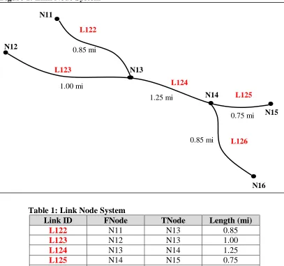
A link node system is a way of defining a network through a series of points and arcs otherwise referred to as nodes and links, respectively [GeoDecisions 1997]. A node is simply defined as a point along an arc that marks the beginning or ending of a link. A link is defined as arc that connects two node points. Therefore, nodes are connected through a series of links.
Consider an example. Figure 1 displays a link node topology and Table 1 defines that same link node topology in tabular form. Each link is provided with a unique identification number, Link ID, and is associated with its FNode and TNode. The FNode (From Node) is a node that defines the “beginning” point of a link. The TNode (To Node) defines the “ending” point of a link. The topology, or connectivity, is defined by matching a link’s TNode to another link’s
FNode or vice versa.
Figure 1: Link Node System
Table 1: Link Node System
Link ID FNode TNode Length (mi)
L122 N11 N13 0.85
L123 N12 N13 1.00
L124 N13 N14 1.25
L125 N14 N15 0.75
L126 N14 N16 0.85
L123
L126 L125 L124
L122
N12
N16 N15 N14
N13 N11
1.00 mi 0.85 mi
1.25 mi
0.75 mi
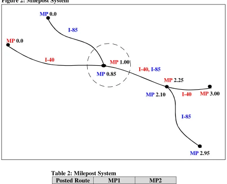
3.2 Milepost System Definition
The milepost system makes use of the posted route system and simply assigns a milepost marker at each node. Figure 2 displays a milepost system and Table 2 defines that milepost system in tabular form. The milepost marker indicates a running sum of distances along a posted route.
MP1 stands for milepost one and indicates the first milepost marker for a given link. MP1 starts at zero at the beginning of each new posted route. It also starts at zero at each county boundary.
MP2 stands for milepost two and denotes the distance to some other location along the roadway such as an intersection.
Figure 2 obviously differs from Figure 1 in the way the nodes are labeled. Instead of being assigned a node number in the Milepost system the nodes are assigned a milepost marker. Note that at some nodes more than one milepost is shown. For example, the node inside the circle has mileposts MP 0.85 and MP 1.00. This indicates that two different posted routes share the node. Posted route I-85 has a milepost of 0.85 miles and posted route I-40 has a milepost of 1.00 miles at that node.
Table 2 is also different from Table 1 in another important way. The use of mileposts in Table 2 eliminates the need to store lengths. Lengths are now calculated rather than stored. Yet at the same time, the concept of links is still implied by the new table structure in that each row in the table mimics a link.
However, problems with the Milepost system may arise as a result of the overlap in road naming conventions. For example, one portion of roadway may have several different posted route names (both I-40 and I-85). If one department or organization refers to the same portion of roadway as I-40 and another department or organization refers to the same portion of roadway as I-85, the system may not have the ability to combine the information gathered to form a complete analysis of the route or link. Furthermore, they may be referring to entirely different portions of I-40 and I-85. Finally, as the names of roads change over time, vital historical data may be lost.
Another problem with the milepost system is that it provides not only two names for any portion of pavement, but it also provides two mileposts. The location identified by MP 2.00 on I-40 is the same location as MP 1.85 on I-85. This is a dangerous situation from the perspective of integrity in a Geographic Information System (GIS) or database.
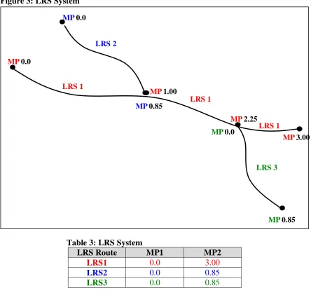
3.3 Linear Referencing System Definition
A linear referencing system is similar to the posted route system in that it groups multiple links together with the same name or ID, but it is unique in that it is linked to the physical pavement rather than to a conceptual route. It is also similar to the milepost system in that it provides each node with a milepost marker instead of a node number. Finally, it also allows for historical analysis because once a link is designated with an LRS ID it is permanent as well as unique.
Additionally, fewer records are needed in the database to describe the actual topology as shown in Table 3. (Note that it is merely coincidence that LRS 2 and LRS 3 are of the same length).
Figure 2: Milepost System
Table 2: Milepost System
Posted Route MP1 MP2
I-40 0.0 1.00
I-40 1.00 2.25
I-40 2.25 3.00
I-85 0.0 0.85
I-85 0.85 2.10
I-85 2.10 2.95
Milepost markers are assigned to nodes and represent the total length of the LRS route up to that point. The total length of the LRS route is the result of the summation of the individual link lengths that comprise the LRS route. Table 3 provides not only the LRS ID, but also MP1 and
MP2. MP1 represents an LRS Route’s very first milepost marker, which should always be 0.00.
MP2 represents an LRS Route’s very last milepost marker and should always equal the sum of all the individual link lengths that comprise the LRS route. Any other location on the roadway can be identified simply by its LRS ID and MPs.
I-40
I-85
I-40 I-40, I-85
I-85 MP 0.0
MP 2.10 MP 1.00
MP 2.95 MP 0.0
MP 3.00 MP 2.25
Figure 3: LRS System
Table 3: LRS System
LRS Route MP1 MP2
LRS1 0.0 3.00
LRS2 0.0 0.85
LRS3 0.0 0.85
4.0 DATABASE SCHEMA
This section presents a portion of the North Carolina Department of Transportation’s Pavement Management Unit (PMU) highway network database schema. The PMU currently uses a link node based referencing system to store all pavement data pertaining to the highway network. The PMU link node database was used as input to generate the LRS routes as output.
4.1 PMU Link Node Referencing System
In the PMU database a node is placed at each intersection. Nodes are also placed at the beginning and ending points of bridges, at railroad crossings, and at county boundaries. Lines (or arcs), referred to as links, connect one node to another with a line and approximate the path of the road network.
The links and nodes are given a statewide unique link number (for all links) and a countywide unique node number (for all nodes). The assignment of these numbers is arbitrary, which means that no numbering pattern can be presumed to be followed. The tables listed below are examples
LRS 1
LRS 3
LRS 1 LRS 1
LRS 2 MP 0.0
MP 0.0
MP 1.00
MP 0.85 MP 0.0
MP 3.00 MP 2.25
of the tables that the Pavement Management Unit uses to implement its link node system. Although the tables represent only a small portion of the complete PMU database, they are the only tables used to define the topology and geometry of the roadway network. It is on these tables that the proposed LRS algorithms operate.
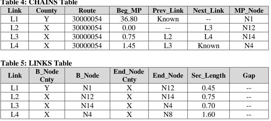
4.1.1 Link Node Spatial Topology Tables
The following table(s) provide the structure of the topological aspects of the link node system. The CHAINS table provides the topology of the roadway network by connecting each link through the use of Prev_Link and Next_Link. Thus, this table assembles individual links together into chains of links that are commonly known as routes.
CHAINS (Link, County, Route, Beg_MP, Prev_Link, Next_Link, MP_Node)
Link – The statewide unique link identification number given to each arc with a beginning and ending node.
County – The county the link is located in.
Route – An 8-digit number that provides information such as route classification (Interstate, US, State, or Secondary road), type of route (Business, Alternate, Regular), Direction, and Posted Route Number.
Beg_MP – Indicates the Posted Route Milepost marker at the beginning node of the link. Prev_Link – The link number of the link directly preceding the current link.
Next_Link – The link number of the link directly following the current link. MP_Node – The node number of the Beg_MP marker.
The LINKS table provides information about each individual link, including its beginning and ending nodes, the county that each is contained within, the length of each link, as well as information about whether it crosses a county boundary. The links are essentially the basic building blocks of routes.
LINKS (Link, B_Node_Cnty, B_Node, End_Node_Cnty, End_Node, Sec_Length, Gap)
Link – The statewide unique link identification number given to each arc with a beginning and ending node.
B_Node_Cnty – A number representing the county where the beginning node is located. B_Node – A countywide unique number representing the beginning of the link.
End_Node_Cnty – A number representing the county where the ending node is located. End_Node – A countywide unique number representing the ending of the link.
Sec_Length – The length of the link (in miles). Gap – The county that a link crosses into.
The following data tables provide a better understanding of the type of information stored in the tables defined above. The information in Table 4, the CHAINS table, and Table 5, the LINKS
table, is a subset of actual data from the PMU’s LINKS and CHAINS tables, respectively. It is included here for illustration only.
Table 4: CHAINS Table
Link County Route Beg_MP Prev_Link Next_Link MP_Node
L1 Y 30000054 36.80 Known -- N1
L2 X 30000054 0.00 -- L3 N12
L3 X 30000054 0.75 L2 L4 N14
L4 X 30000054 1.45 L3 Known N4
Table 5: LINKS Table
Link B_Node
Cnty B_Node
End_Node
Cnty End_Node Sec_Length Gap
L1 Y N1 X N12 0.45
--L2 X N12 X N14 0.75
--L3 X N14 X N4 0.70
--L4 X N4 X N8 1.60
--4.1.2 Challenges Inherent in the PMU Tables
Some observations about the PMU link node system implementation are in order. It is not a pure link node implementation and thus has some unique characteristics and presents some challenges when using it as a basis for generating the LRS routes. For example, at first glance, one may misinterpret the B_Node and End_Node fields in the LINKS table as denoting directionality. However, this is not the case. The B_Node and End_Node identifiers are assigned arbitrarily and do not provide any directional information.
Still, some general directionality can be determined through the highway naming convention adopted nationwide. This naming convention is such that all posted routes with an even number generally run east and west and all posted routes with an odd number generally run north and south.
More specific direction information can be determined from the CHAINS table. This table defines all routes as a chain of multiple links. Following the links in a chain traverses a posted route. A link is listed in the CHAINS table once for each of its assigned posted routes. Therefore, a link may be listed more than once if it lies on the path of more than one posted route.
The Beg_MP provides the mile marker location for one of the nodes of the link in question and is selected as the start (or beginning) node for the link. The Beg_MP value is the sum of all link lengths within the given chain (posted-route) up until that point. The MP_Node is the node identifier where the milepost marker is posted. The MP_Node does not necessarily match a link’s B_Node (in the LINKS table).
In addition to providing information about the beginning point of a link, the CHAINS table also defines the network topology by providing information about a link’s previous and next link. The Prev_Link field is assigned a value of null at the beginning of a posted route chain. Likewise, the Next_Link field is assigned a value of null at the end of a posted route chain. The
Next_Link field is also assigned a value of null when a link encounters a county boundary. The
Prev_Link field is assigned a value of null when the chain crosses the county boundary. Normal chain traversal occurs by following Next_Link after Next_Link until the end of the chain is reached (or Prev_Link to the beginning in reverse). In the case of county boundaries, however, where no next (or previous) link is identified (even though one exists), traversal can still continue. This is done simply by matching on the B_Node and End_Node of the links.
4.2 Study Context
The work described herein makes use of the link node database tables to create the LRS routes by generating LRS IDs for all links in the roadway network. It should be emphasized that it was not a goal of this study to determine whether there was a need for the new LRS system. In a study prior to this it was already concluded that a base LRS system was needed [Kiel 1999]. This work built on that recommendation by providing insight into how to do it. What this study does is provide several LRS configurations to choose from and an interpretation of the analysis results of the various configurations so that the process of choosing an approach is well founded and solidly based.
4.3 General Database Algorithm Constraints
The algorithms that were developed to generate alternative LRS route configurations needed to take into account a number of specific predefined constraints; the constraints limit how the configurations were created. These constraints place restrictions on the definition of the precedence of the road classification scheme for generating LRS IDs, and on the defined coverage area for LRS routes. The constraints apply to all LRS algorithms.
The algorithms are divided into primary route algorithms and secondary route algorithms. A route is classified as a primary route if its posted route number denotes an Interstate, U.S., or State route. A secondary route is any other state-maintained roadway. Primary posted routes are uniquely named throughout the United States for Interstate and U.S. routes and are uniquely named statewide for State routes. This means that Interstate and U.S. posted route numbers do not change when crossing state lines and State posted route names do not change when crossing county lines. Additionally, primary roads may have multiple posted route names assigned to the same pavement (very much unlike the LRS system).
Finally, the LRS coverage area had to be defined. An LRS system can be configured on either a countywide or statewide basis. For primary roads posted routes are defined statewide and, therefore, primary LRS routes should not stop at county lines, but continue on to the state boundary.
The job of the algorithms is to embody various combinations of the constraints to generate different sets of LRS routes. Each algorithm generates a different set of routes by following the PMU database link chains, applying the different set of constraints, individually identifying each route, and assigning it a unique identifier (LRSI, LRS2, etc. are used herein for illustration). Section 4.1 described the PMU database. Section 4.3 (this one) described the constraints. Section 5.0 describes each specific algorithm in detail.
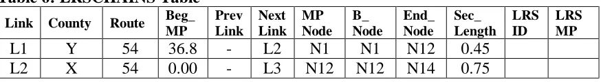
4.4 Database Table
The algorithms use a table with the same format as the LRSCHAINS table. This table is composed of the attributes B_Node, End_Node, and Sec_Length from the PMU LINKS table and all of the attributes from the PMU CHAINS table. Joining the two tables based on the Link
attribute and deleting unnecessary columns created Table 6. (The Route number has been truncated to fit the space provided.)
Table 6: LRSCHAINS Table
Link County Route Beg_
MP
Prev Link
Next Link
MP Node
B_ Node
End_ Node
Sec_ Length
LRS ID
LRS MP
L1 Y 54 36.8 - L2 N1 N1 N12 0.45
L2 X 54 0.00 - L3 N12 N12 N14 0.75
In addition to the attributes that were included as a result of joining the two PMU tables, two new attributes (the LRS ID and the LRS MP fields) were also added. The LRS ID field is used to assign the unique LRS identifier (number) to each link. Links that contain the same LRS ID
comprise an LRS route. The LRS MP is the milepost marker for the new LRS route.
The goal of the algorithms is to use the data from the LRSCHAINS table to identify LRS routes, assign LRS IDs, and to accumulate the mileage (LRS MP) from the information provided in the table. The end result, then, is a complete LRS system that is integrated with the current link node system. Thus, at a later time the link node system can be abandoned and dropped. Thus, the algorithms do two simultaneous things: (1) they determine LRS routes and (2) they provide an automated conversion from the PMU link node system to the LRS system.
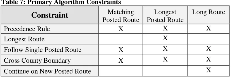
5.0 PRIMARY ALGORITHMS FOR GENERATING LRS IDS
Table 7: Primary Algorithm Constraints
Constraint
MatchingPosted Route
Longest Posted Route
Long Route
Precedence Rule X X X
Longest Route X
Follow Single Posted Route X X X
Cross County Boundary X X X
Continue on New Posted Route X
5.1 Matching Posted Route Algorithm
The Matching Posted Route Algorithm closely resembles the roadway network as it is seen on maps and other printed materials. That is, the LRS routes are chosen to “match” the posted routes.
Within this context one must then further specify the order in which the LRS routes are assigned to the posted routes. The Matching Posted Route algorithm chooses routes based on the posted route numbering. LRS IDs are assigned in a sequential manner to posted routes in the order of lowest to highest posted route number. Therefore, all links that make up I-40 are assigned LRS IDs before I-95, etc. The matching algorithm does not take the length of the route into consideration before assigning LRS IDs. The classification precedence, however, still stands.
Figure 4: LRS Configuration for Matching Posted Route Algorithm
MP 0.00
MP 1.00
MP 0.00
MP 2.25
MP 1.00 LRS 3
LRS 2 LRS 1
LRS 1
LRS 4
MP 0.85
MP 0.00 I-40, I-85 I-85
I-85 I-40
Figure 4 illustrates an example of the resulting route configuration created by using this algorithm. (Note that this figure has been slightly modified from the previous 3 figures through the addition of I-70 to a portion of the linework in lieu of I-40.) As the figure shows, I-40 is assigned an LRS route before I-70 or I-85. Note that the only applied constrains were matching the posted route and ascending order. Length was not considered in any way. As the reader can see, I-85 has been assigned two LRS routes. This is because the pavement occupied by the LRS1 portion of I-85 has already been named. Thus the remaining two segments need to be individually named.
5.2 Longest Posted Route Algorithm
The Longest Posted Route algorithm also generates LRS IDs based on posted route numbers. Therefore, in a manner similar to the Matching Posted Route algorithm discussed in Section 5.1, the Longest Posted Route algorithm also generates an LRS naming pattern that closely resembles the roadway network as labeled on maps and other published materials with the longest posted route LRS IDs generated first. Still, there are noticeable differences.
The Longest Posted Route algorithm can have different constraints depending on the method that one chooses to implement. The only strict constraints defined by the Longest Posted Route algorithm are that it must follow the posted routes and it must assign the longest posted route the current LRS ID. This is clearly different from assigning the LRS ID to the one whose posted route number is numerically the lowest. Thus, an entirely different processing order occurs for the records in the database table.
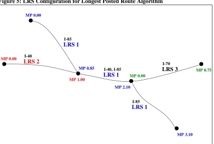
Figure 5: LRS Configuration for Longest Posted Route Algorithm
MP 0.00
MP 1.00
MP 0.00
MP 0.00
MP 3.10
MP 0.75
LRS 1
LRS 3
LRS 2
LRS 1
LRS 1
MP 0.85
MP 2.10 I-40, I-85 I-40
I-85 I-85
The Longest Posted Route algorithm first generates all possible route traversals (while maintaining adherence to posted route numbers) and calculates the total length of each. Once the longest posted route is identified, an LRS ID is assigned to all links within this route. It has thus been named and all of its links are marked as being removed from any further consideration for naming.
Figure 5 illustrates an example of the resulting route configuration created by using the constraints described above (for the Longest Posted Route algorithm). As the figure shows, I-85 is assigned an LRS route before I-40 because it results in a longer overall LRS route. Thus the resulting configuration of Figure 5 is quite different from that of Figure 4.
5.3 Long Route Algorithm
The Long Route algorithm chooses LRS IDs based on something referred to as a "long" route. The Long Route algorithm’s main objective is to produce “long” LRS routes while still adhering to the posted route paths. However, a single LRS may be made up of more than one posted route. Therefore, the LRS routes will closely resemble the roadway posted routes, but they will not necessarily uniquely match the roadway posted routes.
The goal of this algorithm is to generate long LRS routes. This algorithm does enforce adherence to ascending posted route numbering, but the LRS route is allowed to “pick up” another posted route once the end of the current posted route is encountered. The LRS route then follows the new posted route to its end. The resulting routes, therefore, are long. In fact, they are likely to be longer than those generated by the Longest Posted Route algorithm.
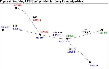
Figure 6: Resulting LRS Configuration for Long Route Algorithm
MP 0.00
MP 1.00
MP 0.00
MP 0.00
MP 3.25
MP 0.75 LRS 3
LRS 2
LRS 1
LRS 1
LRS 1
MP 0.85
MP 2.25 I-40
I-70 I-85
This algorithm enforces the precedence rule so all LRS routes reside within their own posted route category. For example, an LRS route cannot consist of an interstate and US route (all interstate, or all US, or all NC is allowable). It also mandates that LRS routes maintain certain directionality so that an LRS route would not circle back on itself or form a loop.
Figure 6 illustrates an example of the resulting route configuration created by using the constraints described above (for the Long Route algorithm). As the figure shows, LRS 1 starts by selecting I-40 and then continues on I-85 once the end of the posted route chain (I-40) is encountered. When the algorithm encounters a choice between I-70 and I-85 it currently is programmed to arbitrarily choose. Alternatively, it could have been programmed to use specific selection criteria in making this choice. For example, it could have selected the route with the next longest link, the route with the lowest posted route number, the link leading to the largest remaining path, or some other criteria.
5.4 Longest Route Algorithm
Although one of our goals is to obtain the longest LRS routes possible there is no Longest Route algorithm. This is because the difference between the Long Route and Longest Route algorithm results are not significant for primary routes. The reason for this, as previously stated, is that primary posted routes are already as long as they possibly can be. That is, they tend to all run from state border to state border. Because its results are not expected to be significantly different and because (very importantly) it would deviate from following posted routes, this Longest Route algorithm was not developed.
6.0 ALGORITHM COMPARISON
The previous section explored several algorithms for producing the LRS routes. Each algorithm was bound by its own set of constraints, each of which has an impact on the outcome. The following subsections will compare the resulting LRS routes based on a set of measures that were selected as having a bearing on the quality of the resulting LRS configuration. The goal is to evaluate and compare the LRS route configurations generated by the algorithms. The reader might recall that the LRS routes being generated are for two of North Carolina's one hundred counties as was previously discussed in Section 1.2.
In Section 6.1 we simply list and define all of the measures used. In Section 6.2 we report on the values of each measure for each algorithm. Finally, in Section 6.3 we interpret the results and come to some overall determination of how the measures enable us to decide which algorithm best meets our needs.
6.1 Quality Measures for LRS Routes
The following subsections provide a description of one set of quality measures. Most of the quality measure values were obtained by querying and manipulating the LRS tables for each algorithm.
6.1.1 Length of LRS Routes
the route. Once the length of each route was calculated the longest, shortest, average, and median of each LRS route was obtained. Finally, we determined the average length for the shortest 10% of all routes, the next shortest 10% of all routes, etc. These numbers tell us, on average, how short the short routes were, etc.
6.1.2 Number of LRS Routes
The number of LRS routes was determined by identifying the minimum and maximum LRS IDs for each algorithm, subtracting the two, and adding 1. The total number of LRS Routes is important because it determines a maximum number of records that define all of the names (LRS IDs) used in the database. Since LRS ID is a key field, the fewer LRS IDs the faster the processing. In addition to providing the total number of LRS routes for each algorithm, the number of longest routes, long routes, short routes, and shortest routes was also determined. Section 6.2 will provide a more detailed explanation of these terms.
6.2 Quality Measure Results
The following subsections provide results for the quality measures described above. Each quality measure defines a distinct characteristic of the results of each algorithm. In addition to statistical information, graphs and charts were generated along with a detailed description of what each means. Based on the results provided in these sub-sections, an evaluation of each algorithm was formulated and, ultimately, a selection was made.
6.2.1 Length of LRS Routes
The following tables and graphs illustrate, for each algorithm, the values of various measures related to the length of LRS routes. These values show the differences between each algorithm and provide a means to evaluate the results. Included in this is a table that provides the length of the longest LRS route, the length of the shortest LRS route, the average length of all LRS routes, and the median length of all LRS routes. Following the table is a graph and a bar chart for each algorithm that displays additional length data for the routes.
In Table 8 the column headings represent the algorithm names. The rows represent some of the measures that were calculated from the resulting algorithms. The longest and shortest represent the absolute longest and shortest LRS route. The average totals all LRS lengths and divides by the total number of LRS routes. For the median an equal number of LRS routes have a length greater than this value and an equal number have a length less then this value.
Table 8: Length of LRS Routes
Length of LRS
Route Measures
Matching Posted Route
Longest Posted Route
Long Route
Longest 35.84 55.34 37.65
Shortest 0.02 0.02 0.02
Average 13.51 15.27 15.97
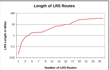
In Figures 7A, 7B, 8, and 9 the vertical axis of each chart or graph represents the length of an LRS Route. The horizontal axis is more complicated. For the graph of Figure 7A, we are plotting a length value for each and every LRS Route. The horizontal axis, then, extends from zero to the largest number of LRS Routes for that algorithm and the result appears to be a continuous string of data points that approximate a curve. To better illustrate the lengths and the number of routes that fall within various length groupings, a logarithmic scale was used to plot the points.
For the bar chart, the approach is different. First, we sort the data by length from the shortest to the longest LRS route. Then the total number of LRS routes is divided into tenths. For example, if there is a total of 100 LRS routes, then each bar represents the average length of 10 LRS routes. Therefore, one bar is plotted for each one-tenth of the total number of LRS Routes. The vertical axis represents the average length of each bar. Note that in all of these figures we are reporting results for only the primary roads in only two counties.
Figure 7A: Matching Posted Route Algorithm Lengths
Length of LRS Routes
0.01 0.1 1 10 100
1 3 5 7 9 11 13 15 17 19 21 23 25
Number of LRS Routes
L
R
S
L
e
n
g
th
i
n
M
il
e
Figure 7B: Matching Posted Route Algorithm Average Lengths
Figure 8: Longest Posted Route Algorithm Average Lengths
Average Length of LRS Routes
0.32 1.33 1.80 2.46 3.99 10.25 21.89
31.88 35.23 42.90
0.1 1 10 100
1 2 3 4 5 6 7 8 9 10
1/10th Number of LRS Routes
A v e ra g e L e n g th i n M il e s
Each 1/10th = 2 Routes
Average Length of LRS Routes
0.32 1.38 1.88 2.80 5.84 8.43 15.04
26.92 31.07 35.43
0.1 1 10 100
1 2 3 4 5 6 7 8 9 10
1/10th Number of LRS Routes
A v e ra g e L e n g th i n M il e s
Figure 9: Long Route Algorithm Average Lengths
6.2.2 Number of LRS Routes
The following tables illustrate, for each algorithm, the values of various measures related to the number of LRS routes. In Table 9 the column headings again represent the algorithm names. The rows are separated into a measures section and a length cutoffs section. The measures identify what is being measured. They are broken into the number of longest, long, short, and shortest routes. These numbers specify the number of routes that fall between 100 and 75 percent (longest), 75 and 50 percent (long), 50 and 25 percent (short), and, finally, 25 and 0 percent (shortest) of the maximum length of the longest LRS route generated by each algorithm. The Length Cutoffs are the absolute values given in units of miles.
Tables 9 is a presentation of relative length measure and it is useful only for understanding the distribution of LRS route lengths for each algorithm. It is not a useful measure for comparing algorithms to each other.
Table 10 identifies the total number of routes within a certain fixed length range. For the primary route algorithms described herein, the length ranges are broken into four equal length groups. (For secondary routes, the length ranges were broken into 10 equal length groups.) Although these two tables provide a means for comparison, it should also be noted that the total number of LRS routes is different for each algorithm.
Average Length of LRS Routes
0.09
1.81 2.49
5.21
8.66
15.92 22.14
28.99 33.62 36.69
0.01 0.10 1.00 10.00 100.00
1 2 3 4 5 6 7 8 9 10
1/10th Number of LRS Routes
A
v
e
ra
g
e
L
e
n
g
th
i
n
M
il
e
Table 9: Number of LRS Routes
Number of LRS
Route Measures
Matching Posted Route
Longest
Posted Route Long Route
Total Number of LRS Routes 26 23 22
Number of Longest Routes 7 (27%) 1 (4%) 6 (27%)
Number of Long Routes 2 (8%) 7 (31%) 3 (14%)
Number of Short Routes 3 (11%) 1 (4%) 3 (14%)
Number of Shortest Routes 14 (54%) 14 (61%) 10 (45%)
Length Cutoffs
100 – 75 % (Longest) 35.84 – 26.88 55.34 – 41.51 37.65 – 28.24 75 – 50 % (Long) 26.88 – 17.92 41.51 – 27.67 28.24 – 18.83 50 – 25 % (Short) 17.92 – 8.96 27.67 – 13.84 18.83 – 9.41 25 – 0 % (Shortest) 8.96 – 0.00 13.84 – 0.00 9.41 – 0
Unlike Table 9, Table 10 presents an absolute length measure and it is useful for understanding the overall length distribution of all the algorithms thereby providing a measure for comparing the algorithms to each other.
Table 10: Number of LRS Routes for Primary Algorithms
Number of LRS
Route Measures
Matching Posted Route
Longest Posted Route
Long Route
Total Number of LRS Routes 26 23 22
Routes > 45 miles 0 (0%) 1 (4%) 0 (0%)
Routes 45 – 30 miles 5 (19%) 6 (26%) 6 (27%)
Routes 30 – 15 miles 4 (15%) 1 (4%) 4 (18%)
Routes 15 – 0 miles 17 (66%) 15 (66%) 12 (55%)
6.3 Algorithm Evaluation Outcome and Analysis
Regarding the number of primary LRS routes, the difference between the Matching and Long Route algorithms was not significant (22 to 23). However, the Longest Posted Route Algorithm does produce fewer LRS routes than the matching Posted Route Algorithm (23 to 26). Although the number is not significantly different, one must remember that our test case was small in comparison to the entire state. Therefore, this seemingly insignificant change in number may prove to be a more substantial difference if tested statewide.
6.4 Visual Inspection
Visual inspections of LRS routes involve displaying each LRS Route configuration using a GIS to create map-like printouts (the reader is referred to Figure 10 for an example of one of the many maps generated by this study). This is an essential part of the evaluation process. It allows one to look at the maps and visually detect errors, both in the algorithm and in the database itself.
As stated previously, the database file that was used in this study was not entirely cleaned. That is, it was not entirely correct. Visual inspection allows one to more easily identify these errors and mistakes, which would otherwise be detected only by laboriously inspecting the LRS system in tabular form. Thus, the route generation process can turn out to be a means to improve the integrity of the database.
For example, consider the Primary Road LRS Routes for the Matching Posted Route Algorithm in Figure 10. LRS Route 14 stops at the New Hanover/Pender County boundary and LRS Route 16 continues into New Hanover. At first glance this appears to be a mistake since it is in fact the same posted route and, therefore, should be assigned the same LRS ID. However, the tabular data has been inspected and a mistake in the database was detected. The algorithm correctly processed the database table, but because the county boundary node for the link was given the wrong number the algorithm stopped at the county boundary. This happened because there was no county boundary node to match with to continue the LRS route.
Referring to the same figure, LRS Route 19 appears to have “jumped” from the upper right corner down to a lower section of the county. Again, this is due to the structure of the database. Within the database, a fictitious link exists along the county boundary for any posted route that crosses into another county and then crosses back into the original county. Therefore, the algorithm used this “link” and continued assigning the LRS ID across it even though this result should not occur.
6.5 Benefits and Obstacles
All of the algorithms provide the same benefit as well as the same result. The result is a set of LRS routes. The benefit is an automated and consistent way to get them. Consistency is an important criteria because the alternative is to do the route generation manually, by human analysts. This approach would undoubtedly introduce a highly undesirable level of both inconsistency and uncertainty in the results. That undermines the purpose of the new roadway information system that the LRS is the base for, and is unacceptable.
All the algorithms evaluated here in could be designed, written, and tested in a reasonable time frame. There was no significant implementation difference that would impact the choice of algorithm. Instead, the quality measures for the results that the algorithms produced were the most significant basis for comparison and evaluation.
result. Unfortunately one of the reasons for creating a new system like the LRS is that the existing databases are in very poor condition. Thus, paradoxically, the big obstacle to a good route system is a lack of good information about the system to start with!
To take this a step further we might discover that the number of errors in a location-based database from a typical state highway department is so large that an implementation of a new LRS may not be feasible using that database. If this is the case, that DOT must simply start over from scratch. If the highway network, or the data describing it, are either highly out-of-date or invalid (inaccurate in either case) one cannot use it. But in our study the errors in the original database are not that large, they are being corrected, and the algorithms are well founded and will produce acceptable results.
7.0 CONCLUSIONS AND RECOMMENDATIONS
The North Carolina Department of Transportation LRS model study (Kiel 1999) suggested that long LRS routes and that keeping the number of LRS routes to a minimum is significantly important. Combining these two goals with the results of the testing conducted herein we draw a number of conclusions and make the following preliminary observations.
7.1 Algorithm Selection
For primary routes it appears that the most promising approach is that encoded by the Longest Posted Route Algorithm. From the test cases provided by the NC DOT (New Hanover and Pender Counties) this algorithm produces the longest routes overall and has the fewest LRS routes compared to the other algorithms tested.
It must be noted that a more comprehensive test case is essential to verifying this preliminary conclusion. Still, this recommendation is not made lightly. An examination of Table 8 shows consistency with what we would have expected to find. The Matching Posted Route algorithm and Longest Posted Route algorithm are both algorithms that force the LRS routes onto posted routes. Interstate and US routes are generally statewide in length. Thus, to match them is to automatically get a long route. Additionally, a similar result occurs for US and NC routes.
7.2 Transition and Correlation
It is expeditious to consider the LRS in terms of the existing posted route system which provides the largest implementation base in legacy databases. To the extent that the LRS can “somewhat” mirror the posted route system without sacrificing any of the advantages of the LRS approach, it should do so. As a result, the transition from posted routes to LRS routes should be relatively easy and natural for those working at the level of the base referencing system. For all others the LRS is invisible, that is, they need not know that the internal representation of the roadway network is the LRS. Rather, they are simply performing design and analysis with useful computing tools that hide numerous implementation details.
7.3 Additional Testing
produce the anticipated results. It is recommended that the algorithms be tested on a four-county group, internal to the state, with no river bordering the county boundary. This would verify the county boundary tests more accurately than the current New Hanover and Pender test cases that had these disadvantages.
Once the algorithms have been tested using the suggested four county grouping, the results of the quality measures should again be carefully analyzed. If these results are the same as the results from this study, then the recommended algorithm(s) should be chosen and run on the entire state. However, if the results do not produce the same outcome as this study, all algorithms should be reviewed, appropriate changes should be made, and a different recommendation may be in order. Finally, the algorithms need to be executed statewide to generate the LRS network.
11.0 REFERENCES
Adams, T., Chou, H.L., Sun, F., and Vonderohe, A., “Results of a Workshop on a Generic Data Model for Linear Referencing Systems,” AASHTO Symposium on GIS in Transportation, Sparks, Nevada, Pages 1-34 (April 1995).
Butler, J.A. and Dueker, K.J., “GIS-T Enterprise Data with Suggested Implementation Choices,” Center for Urban Studies, Portland State University, Portland, Oregon, Pages 1-23 (November 1996).
Dueker, K. J. and Butler, J. A. GIS-T Enterprise Data Model with Suggested Implementation Choices, Center for Urban Studies, School of Urban and Public Affairs, Portland State University, Portland, OR, 1997.
GeoDecisions (A Division of Gannett Fleming, Inc.) (1997). "Linear Referencing Systems -Review and Recommendations for GIS and Database Management Systems," Technical Report, NCDOT, Raleigh, NC, June.
Kiel, D., Rasdorf W., Shuller, E. and Poole, R., "An LRS Model for NCDOT," Transportation Research Record, Number 1660, National Research Council, Washington, D.C., Pages 108-113 (1999).
Miles, S.B. and Ho, C.L., “Applications and Issues of GIS as a Tool for Civil Engineering Modeling,” Journal of Computing in Civil Engineering, Volume 13, Number 3, July 1999.
NCHRP, “Development of System Application Architectures for Geographic Information Systems in Transportation,” Research Results Digest, National Cooperative Highway Research Program, Number 221, Pages 1-20 (March 1998).
Rasdorf, W. J., "A Spatial and Attribute Database Schema Design for Traffic Survey Data," Technical Report, NCDOT (December 1999).
Rasdorf, W. J., "The Conceptual Universe Database Schema: Design Issues and Decisions," Technical Report, NCDOT (August 1999).
Sherk, S. A. and Rasdorf, W. J., "Unified Database Schema for North Carolina Department of Transportation," Technical Report, NCDOT (June 1998).
Vonderohe, A., Chou, C., Sun, F., and Adams, T, "A Generic Data Model for Linear Referencing Systems," NCHRP Research Results Digest, Transportation Research Board, National Research Council, Washington, D.C., Number 218, (September. 1997).
Vonderohe, A., Adams, T., Chou, C., Bacon, M., Sun, F., and Smith, R, "Development of System and Application Architectures for Geographic Information Systems in Transportation," NCHRP Research Results Digest, Transportation Research Board, National Research Council, Washington, D.C., Number 221, (March 1998).