ABSTRACT
DONG, LIN. Semiparametric Methods for Decision Making and Causal Effect Generalization. (Under the direction of Dr. Eric Laber and Dr. Shu Yang).
©Copyright 2019 by Lin Dong
Semiparametric Methods for Decision Making and Causal Effect Generalization
by Lin Dong
A dissertation submitted to the Graduate Faculty of North Carolina State University
in partial fulfillment of the requirements for the Degree of
Doctor of Philosophy
Statistics
Raleigh, North Carolina 2019
APPROVED BY:
Dr. Eric Laber
Co-chair of Advisory Committee
Dr. Shu Yang
Co-chair of Advisory Committee
Dr. Rui Song Dr. Yair Goldberg
External Member
DEDICATION
BIOGRAPHY
ACKNOWLEDGEMENTS
I would like to express my deepest appreciation to my advisors. I am deeply indebted to Dr. Eric Laber for his continuous support and guidance. He is a great advisor and leader, who has been providing me and Laber-Labs with valuable resources. I thank him for giving me the chances to tackle various tasks and challenges, which greatly broaden my horizon. I would like to extend my deepest gratitude to Dr. Shu Yang for her kindly guidance and patience that cannot be underestimated. She is a great scholar and is always prompt on answering my questions. The completion of my dissertation would not have been possible without the support of them.
I would like to extend my sincere thanks to my committee members, Dr. Rui Song, Dr. Yair Goldberg and Dr. Jamian Pacific for their advises and time devoted to serve in the committee. I must also thank Dr. Vijay Nair and Dr. Joel Vaughan at Wells Fargo for their constructive advises in the structured neural network project. I would like to thank Dr. Shannon Holloway for helping me polish the writing of my dissertation. I also wish to thank Dr. Sujit Ghosh for his guidance in a biosimilar project.
The department of statistics at North Carolina State University is a great place to conduct collaborative research. Many thanks also to the entire faculty and staffs in the department for offering such a friendly environment.
I owe my long overdue thanks to my professors in HKBU. My gratitude goes to Dr. Lixing Zhu, Dr. Man-Lai Tang and Dr. Xiaonan Wu for encouraging me to pursue a doctoral degree and their recommendations.
I want to express my sincere appreciation to my Laber-Labs lab-mates for the valuable discussions we had over the years. Special thanks to the friends I met during my graduate study and internships. We had a lot of good-times together.
TABLE OF CONTENTS
LIST OF TABLES . . . vii
LIST OF FIGURES . . . ix
Chapter 1 Introduction . . . 1
1.1 Semiparametric methods . . . 1
1.2 Overview of research work . . . 2
Chapter 2 Dynamic treatment regimes with missing data . . . 5
2.1 Introduction . . . 5
2.2 Setup and notation . . . 7
2.3 Estimation with complete data . . . 9
2.3.1 Q-learning with complete data . . . 10
2.3.2 Outcome weighted learning with complete data . . . 12
2.4 Estimation with incomplete data . . . 18
2.4.1 Missingness mechanism . . . 18
2.4.2 Inverse probability weighted estimating equations . . . 19
2.4.3 Augmented inverse probability weighted estimating equations . . . 20
2.5 Simulation and Data Application . . . 22
2.5.1 Simulation Studies . . . 22
2.5.2 CATIE Trial Analysis . . . 24
2.6 Discussion . . . 30
Chapter 3 Integrative analysis of randomized clinical trials with real world evidence studies . . . 31
3.1 Introduction . . . 31
3.2 Basic setup . . . 34
3.2.1 Notation: causal effect and two data sources . . . 34
3.2.2 Identification assumptions . . . 35
3.2.3 Existing estimation methods . . . 37
3.3 Calibration weighting estimators . . . 38
3.4 Semiparametric efficient estimator whenY and A are available in RWE . . . 41
3.4.1 Augmented calibration weighting estimator . . . 41
3.4.2 Semiparametric models by the method of sieves . . . 45
3.5 Simulation . . . 48
3.6 Real data application . . . 55
3.7 Concluding remarks . . . 57
Chapter 4 Model building with structured neural networks . . . 58
4.1 Introduction . . . 58
4.3 Structured neural networks . . . 61
4.3.1 Architecture of structured neural networks . . . 61
4.3.2 Regularization . . . 65
4.3.3 Computation . . . 66
4.4 Prediction error based model ranking . . . 66
4.4.1 Prediction error . . . 66
4.4.2 Hypothesis test . . . 67
4.5 Simulation studies . . . 70
4.5.1 Comparative study of sNN and semiparametric regression models . . . 70
4.5.2 Simulation studies on model ranking . . . 71
4.6 Concluding remarks and future work . . . 74
BIBLIOGRAPHY . . . 81
APPENDICES . . . 94
Appendix A Appendix for Chapter 2 . . . 95
A.1 IPWCC estimating equations . . . 95
A.2 AIPWCC estimating equations . . . 96
A.3 Simulation settings . . . 97
A.4 Proof of Theorem 1 . . . 97
A.5 Proof of Theorem 2 . . . 99
Appendix B Appendix for Chapter 3 . . . 102
B.1 Additional treatment calibration . . . 102
B.2 Proofs . . . 104
B.2.1 Proof of Theorem 3 . . . 104
B.2.2 Proof of Theorem 4 . . . 111
B.2.3 Proof of Theorem 5 . . . 114
B.2.4 Proof of Theorem 5 and Theorem 6 . . . 116
B.3 Conditions for the sieves estimator . . . 117
B.4 Additional simulation study . . . 118
B.4.1 Comparison of the CW estimators . . . 118
B.4.2 Increased sample sizes . . . 119
Appendix C Appendix for Chapter 4 . . . 125
C.1 sNN specifications . . . 125
LIST OF TABLES
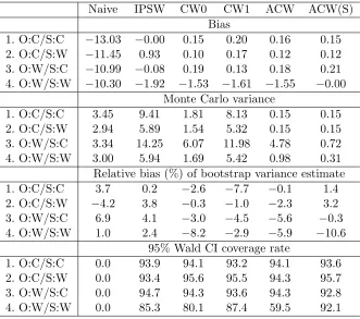
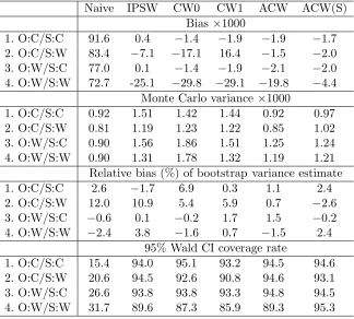
Table 2.1 Cross-validated value estimates of the optimal regimes estimated using different methods. . . 29 Table 3.1 Simulation results forcontinuous outcome: bias of point estimates, Monte
Carlo variance, relative bias of bootstrap variance estimate, and the coverage rate of 95% Wald confidence interval. . . 51 Table 3.2 Simulation results forbinary outcome: bias of point estimates, Monte Carlo
variance, relative bias of bootstrap variance estimate, and the coverage rate of 95% Wald confidence interval. . . 53 Table 3.3 Number of patients by treatment of the CALGB 9633 trial sample and the
NCDB sample. . . 55 Table 3.4 Covariate and outcome means comparison of the CALGB 9633 trial sample
and the NCDB sample. . . 57 Table 3.5 Point estimate, standard error and 95% Wald confidence interval of the
causal risk difference between adjuvant chemotherapy and observation based on the CALGB 9633 trial sample and the NCDB sample. . . 57 Table 4.1 Summary of structured neural networks and their model structures. . . . 62 Table 4.2 Comparison on MSE (S.E.) of sNN with semiparametric regressions: (a).
SIM-Net verses PPR with one ridge function; (b). AM-Net verses GAM; (c). AIM-Net verses PPR with three ridge functions. . . 78 Table 4.3 Summary of Case 1: point estimate of prediction risk, 95% coverage of the
Wald-type confidence intervals for each model; mean of p-values, empirical type I error rate and power for each pairwise comparison w/o Holm adjust-ment; percentage of the estimated best set contains the true best model w/o Holm adjustment and the average length of the the estimated best set. 79 Table 4.4 Summary of Case 2: point estimate of prediction risk and 95% coverage of
the Wald-type confidence interval; mean ofp-value, empirical type I error rate and power w/o Holm adjustment; percentage of the estimated best set contains the true best model w/o Holm adjustment and the average length of the the estimated best set. . . 79 Table 4.5 Summary of Case 3: point estimate of prediction risk and 95% coverage of
the Wald-type confidence interval; mean ofp-value, empirical type I error rate and power w/o Holm adjustment; percentage of the estimated best set contains the true best model w/o Holm adjustment and the average length of the the estimated best set. . . 80 Table B.1 Simulation results forcontinuous outcome with population sizeN = 500000:
LIST OF FIGURES
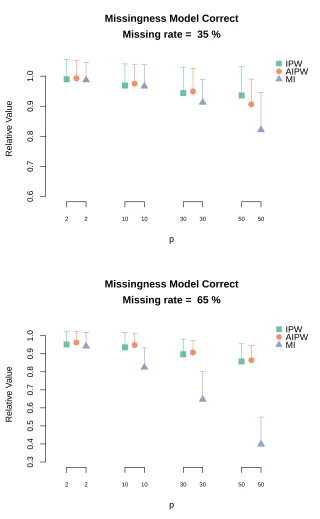
Figure 2.1 Relative value of Q-learning with IPWCC estimator, AIPWCC estimator and MI when the missingness model is correctly specified. The length of the corresponding vertical bar is the Monte Carlo standard deviation of the relative value estimates . . . 25 Figure 2.2 Relative value ofoutcome weighted learning with IPWCC estimator,
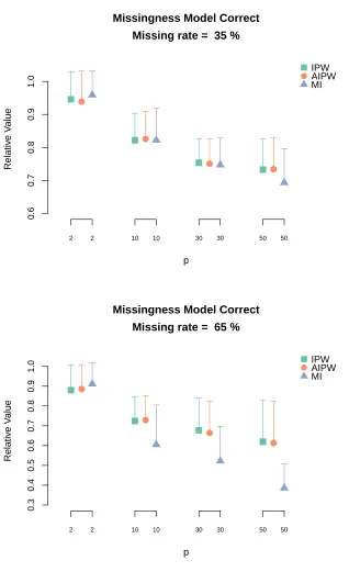
AIP-WCC estimator and MI when the missingness model is correctly specified. The length of the corresponding vertical bar is the Monte Carlo standard deviation of the relative value estimates. . . 26 Figure 2.3 Relative value of Q-learning with IPWCC estimator, AIPWCC estimator
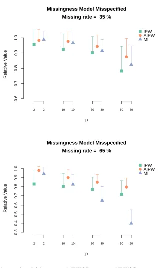
and MI when the missingness model is misspecified. The length of the corresponding vertical bar is the Monte Carlo standard deviation of the relative value estimates. . . 27 Figure 2.4 Relative value ofoutcome weighted learning with IPWCC estimator,
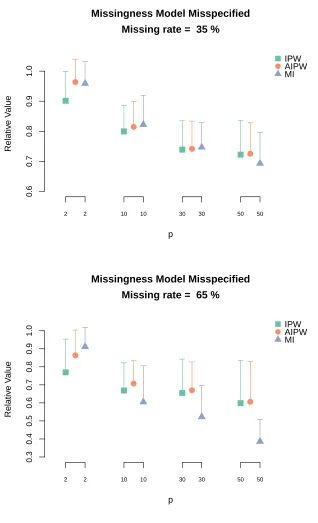
AIP-WCC estimator and MI when the missingness model is misspecified. The length of the corresponding vertical bar is the Monte Carlo standard deviation of the relative value estimates. . . 28 Figure 2.5 Missiningness pattern of CATIE study after cleaning. . . 29 Figure 3.1 Demonstration of the sampling and treatment assignment regimes for the
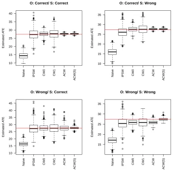
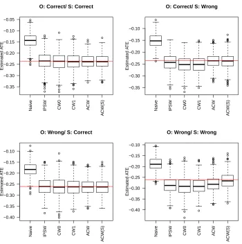
RCT and RWE samples within the target population. . . 36 Figure 3.2 Boxplot of estimators forcontinuous outcomeunder four model specification
scenarios. . . 52 Figure 3.3 Boxplot of estimators for binary outcome under four model specification
scenarios. . . 54 Figure 4.1 Architecture of a subnetwork with 5 hidden layers. . . 62 Figure 4.2 Network architectures of (a) SIM-Net, (b) AM-Net, and (c) AIM-Net. . . 64 Figure 4.3 From top to bottom, partially ordered simple to complex structures. . . . 65 Figure 4.4 Empirical distribution and fitted density of prediction risks based on the
validation dataset of Case 1. . . 75 Figure 4.5 Empirical distribution and fitted density of prediction risks based on the
validation dataset of Case 2. . . 76 Figure 4.6 Empirical distribution and fitted density of prediction risks based on the
validation dataset of Case 3. . . 76 Figure 4.7 Illustration of the proposed visualization tool. . . 77 Figure B.1 Boxplot of estimators under four model specification scenario: ˆτCW0 is
worsen than ˆτCW1. . . 120 Figure B.2 Boxplot of estimators for continuous outcome with population sizeN =
CHAPTER
1
INTRODUCTION
1.1
Semiparametric methods
data integration and machine learning and are the focus of this dissertation.
1.2
Overview of research work
A summary of the chapters that follow is given here as an overview of the research work included in this dissertation.
Chapter 2 is dedicated to semiparametric methods in the context of missing data. We explore this scenario by application to the subject area of dynamic treatment regimes (DTRs), an area of growing importance in the age of precision medicine. Generally speaking, dynamic treatment regimes operationalize precision medicine as a sequence of decision rules, one per stage of clinical intervention, that map up-to-date patient information to a recommended intervention. Of primary importance in this field is the identification of an ”optimal” treatment regime, i.e., one that maximizes a mean utility function when applied to the population of interest. Current methods for estimating an optimal treatment regime assume that the data is fully observed, which rarely occurs in practice. A common approach to overcome this shortcoming of available data is to use multiple imputation and pool estimators across imputed (complete) datasets. However, this approach requires estimating the joint distribution of patient trajectories, which can be high-dimensional, especially when there are multiple stages of intervention. To avoid the underlying modeling step required to obtain complete data, we propose a weighted estimating equation based approach to estimate optimal treatment regimes. Our approach applies to a broad class of estimators including Q-learning and a generalization of outcome weighted learning, which are among the most popular estimators of an optimal treatment regime. In addition, we establish consistency under mild regularity conditions and demonstrate the advantages of our proposed methods in finite samples using simulation experiments and application to a schizophrenia study.
we refer to as the target population. Another data source, called real world evidence (RWE) studies, often include large samples that are representative of a target population, but such studies are often observational and subject to complex confounding. In Chapter 3, we leverage the complementing features RCT and RWE to estimate the average treatment effect of the target population. First, we propose a calibration weighting estimator that uses only covariate information from the RWE study. Because this estimator enforces the covariate balance between the RCT and RWE study, the generalizability of the trial-based estimator is improved. We further propose an augmented calibration weighting estimator that can be applied in the event that treatment and outcome information is also available from the RWE study. This estimator achieves a semiparametric efficiency bound that we derived under the identification and outcome mean function transportability assumptions when the nuisance models are correctly specified. To resolve the misspecification issue associated with parameteric approaches, a data-adaptive nonparametric sieve method is provided as an alternative. The sieve method guarantees good approximation of the nuisance models. We establish related asymptotic results under mild regularity conditions. Finite sample performances of the proposed estimators are verified in simulation studies. Finally, we apply our proposed methods to estimate the effect of adjuvant chemotherapy in early-stage resected non-small-cell lung cancer, where we utilize the data from trial CALGB 9633 and a sample from the National Cancer Database.
CHAPTER
2
DYNAMIC TREATMENT REGIMES WITH MISSING DATA
2.1
Introduction
Dynamic treatment regimes operationalize clinical decision making as a sequence of decision rules, one per stage of intervention, that map current patient information to a recommended intervention (Murphy, 2003; Robins, 2004).An optimal treatment regime maximizes the mean utility if applied to select interventions in the patient population of interest (for alternative definitions of optimality, see Kosorok & Moodie, 2015; Linn et al., 2017; Wang et al., 2018). Optimal treatment regimes have been estimated across a wide range of application areas including anticoagulation (Henderson et al., 2010; Barrett et al., 2014; Rich et al., 2014), cancer (Wang et al., 2012b; Xu et al., 2019), mental disorders (Nahum-Shani et al., 2012; Laber et al., 2014a; Zhang et al., 2017), and HIV (Laan & Petersen, 2007; Petersen et al., 2012; Young et al., 2011). In these and nearly all other biomedical application areas, the observed data are subject to missingness, which can include missing measurements, treatments, and outcomes (Shortreed et al., 2014; Kosorok & Moodie, 2015).
data. This body of research includes: approximate dynamic programming methods like Q- and A-learning (Murphy, 2003; Robins, 2004; Blatt et al., 2004; Murphy, 2005a; Moodie et al., 2007; Schulte et al., 2014) and its many variants (e.g., Zhao et al., 2009; Goldberg & Kosorok, 2012; Lu et al., 2013; Moodie et al., 2014; Tian et al., 2014; Laber et al., 2014b; Zhou & Kosorok, 2017; Jeng et al., 2018; Shi et al., 2018; Kosorok & Laber, 2019, and references therein) ; direct-search methods including outcome weighted learning (Orellana et al., 2010; Zhang et al., 2012a; Zhao et al., 2012; Zhang et al., 2013; Zhao et al., 2014; Zhao et al., 2015; Zhou et al., 2017; Athey & Wager, 2017; Zhang et al., 2017; Zhang & Zhang, 2018; Liu et al., 2018; Luckett et al., 2018); and model-based planning via g-computation (see Robins, 1997; Yu & Laan, 2002; Xu et al., 2016; Xu et al., 2019; Guan et al., 2018; Laber et al., 2018, and references therein). Because these methods require complete data, it is often necessary to employ methods to address missing data. A common approach is to apply multiple imputation to complete the data, compute a given estimator of an optimal regime on each of the imputed data sets, and then aggregate these estimators. e.g., by averaging or voting (Almirall et al., 2016; Lu et al., 2016; Ertefaie et al., 2016; Nahum-Shani et al., 2017; Kilbourne et al., 2018; Kidwell et al., 2018). Though estimation of an optimal treatment regime is often but one part of a suite of secondary analyses, the requirement to develop a complete dataset is convenient as it can be used for a variety of other analyses.
standard arguments of semiparametric efficiency theory establishes a double robustness property for this class of estimators (e.g., Tsiatis, 2007). We show that augmented weighting performs favorably as compared to multiple imputation and to simple inverse probability weighting in simulation examples. These results suggest that investigators should give serious consideration to using weighting methods as an alternative to multiple imputation in the context of estimating optimal treatment regimes in practice.
The remainder of this chapter is organized as follows. In Section 2.2, we set notation and define an optimal treatment regime using potential outcomes. In Section 2.3, we describe a class of estimators of an optimal treatment regimes for use with complete data; this class includes Q-learning and outcome weighted learning as special cases. In Section 2.4, we derive an augmented inverse probability weighted estimator for the proposed class of estimators that applies under a monotone missingness pattern. In Section 2.5, we present simulation examples and an application to data from a sequential multiple assignment randomized trial on schizophrenia. A brief discussion of future work is given in Section 2.6.
2.2
Setup and notation
We consider longitudinal data arising from an observational study or a sequential multiple assignment randomized trial (SMART, Lavori & Dawson, 2004; Murphy, 2005b; Kidwell, 2014). The complete data are assumed to be of the form
X1i, A1i,X2i, A2i, . . . ,XT i, AT i, Yi n i=1, which comprise n independent replicates of (X1, A1,X2, A2, . . . ,XT, AT, Y), where: T is the
number of treatment stages,X1 ∈Rp1 is baseline patient information andXt∈Rpt is information
collected during stage (t−1) for t = 2, . . . , T, At ∈ At = {−1,1} is the treatment assigned
during stage t = 1, . . . , T, and Y ∈ Y = R is the terminal outcome coded so that higher
restriction to allow for a simple and unified notation.
DefineH1 =X1, and recursively define Ht= (Ht−1, At−1,Xt) fort= 2, . . . , T. Thus, Ht is
the information available to the decision maker at timet= 1, . . . , T. LetHtdenote the support of
Ht, and for eachht∈Ht, define Ψt(ht)⊆At to be the set of allowable treatments for a patient
presenting with historyHt=ht at time t. A treatment regime in this context is a sequence of
maps,πππ= (π1, . . . , πT), withπt:Ht→At andπt(ht)∈Ψt(ht) for allht∈Ht and t= 1, . . . , T.
Underπππ, a patient with history Ht=ht at time twould be recommended to receive treatment
πt(ht). Let Π denote the space of all feasible regimes. An optimal treatment regime, sayπππopt ∈Π,
maximizes the mean outcome if applied to the population of interest. We formalize this definition using potential outcomes (Rubin, 1978; Neyman, 1923).
For each t = 1, . . . , T, define at = (a1, . . . , at). Let H∗t(at−1) denote the potential history
under treatment sequenceat−1, and let Y∗(aT) denote the potential outcome under treatment
sequence aT. Therefore, the set of all potential outcomes is
W∗ ={H∗t(at−1), Y∗(aT) : at∈Ψt{H∗t(at−1)}, t= 1, . . . , T},
where we have defined H∗1(a0)≡H1. Let 1(·) be the indicator function. The potential outcome under a regimeπππ∈Π is
Y∗(πππ) =X
aT
Y∗(aT) T Y
v=1
1[πv{H∗v(av−1)}=av].
Define the value of regimeπππ to beV(πππ) =EY∗(πππ), i.e., the marginal mean outcome if all subjects
were assigned treatment according toπππ. The optimal regime,πππopt∈Π, satisfies V(πππopt)≥V(πππ) for allπππ ∈ Π. To identifyπππopt in terms of the data-generating model, we make the following assumptions: (i) consistency, Ht = H∗t(At−1) for t = 2, . . . , T and Y = Y∗(AT), (ii) strong
ignorability, At⊥W∗
Ht for t= 1, . . . , T, and (iii) positivity, P(At= at|Ht= ht)>0 for all
literature (see Robins, 2004; Chakraborty & Moodie, 2013; Schulte et al., 2014; Kosorok & Moodie, 2015, for additional discussion). Hereafter, we implicitly assume that these conditions hold.
2.3
Estimation with complete data
In this section, we review estimation of an optimal treatment regime when the data are completely observed. We consider a class of estimators that are representable as solutions to a set of estimating equations. This class is quite broad and includes most of the estimators commonly used in practice. To illustrate this point, we show in the Appendix that Q-learning and a generalization of outcome weighted learning belong to this class.
We consider treatment regimes of the form πππβββ = {π1(·;βββ1), . . . , πT(·;βββT)} in which the
decision rules composing the regime are indexed by parametersβββ = (βββT 1, βββ
T 2, . . . , βββ
T
T)
T∈B, where
B is a normed linear space with norm|| · ||B. For example, one might consider linear decision rules of the form πt(ht;βββt) = sign βββTtht,0
, where ht,0 is a feature vector constructed fromht
and sign(u) is 1 ifu is positive and−1 otherwise. We do not exclude the case in whichβββtincludes
nuisance parameters so thatπt(·:βββt) depends only on a subvector of βββt; however, we do not
make any special distinction for such nuisance parameters as it is not important for our purposes. We assume that an estimatorβββbn= (ββbβ
T
1,n, . . . ,βββb
T
T ,n)T ofβββ is constructed by solving the estimating
equation
Pnmn(HT, AT, Y;βββ) = 0 (2.1)
over βββ ∈ B, where Pn denotes the empirical measure, and mn : HT ×AT ×Y → RJ. The
dependence of mn on nis to allow for regularization or other factors that may vary with the
t= 1, . . . , T rather than the complete dataST+1 ,(HTT, AT, Y)T. For t= 1, . . . , T define Jtto
be the indices of mn such that mn,j depends onST+1 only through St, i.e.,
Jt={1≤j≤J : mn,j(hT, aT, y;βββ) =men,j(ht, at;βββ) for somemen,j :Ht×At→R},
andJT+1are the indices that rely on the complete data. Under this representation, the estimation equation in (2.1) can be equivalently expressed as
Pnmen,j(St;βββ) = 0 for all j∈Jt, t= 1, . . . , T + 1. (2.2)
We will exploit this representation to use more of the observed data in constructing weighted complete case estimators in Section 2.4.
Let βββ∗n denote the population analog ofββbβn, i.e., the solution to (2.2) with Pn replaced by
P. We say thatββbβn is consistent if ||ββbβn−βββ∗n||B converges to zero in probability. Because our
objective is not to propose new estimators of an optimal treatment regime, we will assume that the estimating equation has been suitably constructed to ensure consistency under the data-generating model in the complete data case and avoid stating specific conditions under which such consistency holds. Giving such general conditions would be cumbersome; for example, the conditions under which Q-learning with linear models is consistent are quite different from those under which kernel-based outcome weighted learning is consistent. Before describing how to adjust the estimating equations to accommodate missing data we first briefly recount how to expressQ-learning and outcome weighted learning in the form given in (2.1).
2.3.1 Q-learning with complete data
2018). The basis for Q-learning is the dynamic programming characterization of an optimal regime. DefineQT(hT, aT) =E(Y|HT =hT, AT =aT), and recursively fort=T−1, T−2, . . . ,1
define Qt(ht, at) = Emaxat+1∈Ψt+1(Ht+1)Qt+1(Ht+1, at+1)
Ht = ht, At = at . It follows from
dynamic programming that the optimal regime satisfiesπoptt (ht) = arg maxat∈Ψt(ht)Qt(ht, at) (Bellman, 1957). Let Qt(ht, at;βββt) denote a posited class of models for Qt(ht, at) indexed by
β
ββt∈Bt for t= 1, . . . , T. The induced class of treatment regimes is thus of the form πt(ht;βββt) =
arg maxat∈Ψt(ht)Qt(ht, at;βββt) (Zhang et al., 2012b). IfBt=R
pt andQ(h
t, at;βββt) is differentiable
inβββt for all ht, at∈Ht×At, thenβββbT ,n solves
Pn{Y −QT(HT, AT;βββT)} ∇βββTQT(HT, AT;βββT) = 0, (2.3)
and for t=T −1, T −2, . . . ,1 the estimatorsβββbt,n solve
Pn
max
at+1∈Ψt(Ht+1)
Qt+1(Ht+1, at+1;βββbt+1,n)−Qt(Ht, At;βββt)
∇βββtQt(Ht, At;βββt) = 0. (2.4)
Thus, the estimatorββbβnis obtained by solvingPnmn(βββ) = 0, wheremnis constructed by stacking
(2.3) and (2.4) forT−1, . . . ,1 so thatβββbn is a root of
Pn
{Y −QT(HT, AT;βββT)} ∇βββTQT(HT, AT;βββT)
max aT∈ΨT(HT)
QT(HT, aT;βββT)−QT−1(HT−1, AT−1;βββT−1)
∇βββT−1QT−1(HT−1, AT−1;βββT−1)
. . .
max a2∈Ψ2(H2)
Q2(H2, a2;βββ2)−Q1(H1, A1;βββ1)
∇βββ1Q1(H1, A1;βββ1)
.
The estimated optimal decision at staget is thusπbn,t(ht) = arg maxat∈Ψt(ht)Qt(ht, at;βββbt,n). Similar expressions can be obtained for nonparametric variants ofQ-learning (Zhao et al., 2009; Moodie et al., 2014; Zhang et al., 2017). For the purpose of illustration, we briefly describe kernel ridge regression forQ-learning. Suppose thatHt⊆Rpt for allt= 1, . . . , T. For eacht, let
Kt:Rpt×Rpt →Rbe symmetric and positive definite and write Ht to denote the corresponding
Shawe-Taylor, 2000; Moguerza & Mu˜noz, 2006; Berlinet & Thomas-Agnan, 2011; Nosedal-Sanchez et al., 2012). To approximate QT within HT, one solves for eacha∈ {−1,1}
b
QT ,n(·, a) = arg min fa∈HT
Pn1AT=a{Y −fa(HT)} 2+λ
T ,a,n||fa||2HT, (2.5)
whereλT ,a,n≥0 is a tuning parameter. For eacha∈ {−1,1}defineIT,a={i : AT ,i=a}to be the
subset of patients to receive treatmentaat time T and define ZTT ,a(hT) ={KT(HT ,i,hT)}i∈IT ,a.
It follows that QbT ,n(hT, aT) =ZTT ,a
T(hT)βββbT ,a,n, whereβββbT ,a,n is a solution of
Pn1AT=aT
n
Y −(1 +λeT ,a,n)ZTT ,a
T(HT)βββT,a
o
ZT,aT(HT) = 0.
Notice that in the previous estimating equation, we have replaced λT ,a,n by eλT ,a,n to reflect
in re-writing the estimator the penalty has been scaled by the number of subjects receiving treatmentaT. Constructing Zt,at(ht) analogously for t=T −1, T −2, . . . ,1, one can construct estimatorsQbt,n(ht, at) =ZTt,a
t(ht)βββbt,a,n whereβββbt,a,n is a solution of
Pn1At=at
max
at+1∈Ψt+1(HT+1)
b
Qt+1,n(Ht+1, at+1)−(1 +λet,a,n)ZTt,a
tβββt,a
Zt,at(Ht) = 0.
The preceding estimating equations can be stacked to obtain a single estimating equation; see Zhang et al. (2017) for additional details.
2.3.2 Outcome weighted learning with complete data
(2012) and has since been generalized to multi-stage decisions (Zhao et al., 2015) and undergone a number of other modifications and refinements (Zhao et al., 2014; Chen et al., 2016; Zhou et al., 2017; Liu et al., 2018; Qi & Liu, 2018a; Qi et al., 2018b).
We consider a variant of outcome weighted learning that uses a convex relaxation of the augmented inverse probability weighted estimator of the marginal mean outcome (Zhang et al., 2013; Liu et al., 2018; Zhao et al., 2019a). We use a backwards recursive procedure (see Zhao et al., 2015) to extend the single-stage procedure proposed by Zhao et al. (2019a) to multiple-stages; while this is our not main methodological contribution, it may of be interest in its own right (see Zhang & Zhang, 2018; Davidian et al., 2019, for additional details).
We describe the estimator as a sequence of models fit, each indexed by their own parameters, before stacking the models and parameters into a single estimating equation. To ease bookkeeping and clarify development, we begin by usingηηη = (ηηηT
1, . . . , ηηηTT)
T solely to index the decision rules and use θ= (θT
1, . . . ,θTT)T to index nuisance models; we later pool these into a single collection
of parameters,βββ = (βββT
1, . . . , βββTT)T, to match the notation used in our general framework. For
simplicity, we assume linear decision rules of the form πt(ht;ηηηt) = sign(ηηηTtht,0), where ht,0 is known feature vector constructed fromht. Furthermore, letQT(hT, aT;θT) be a posited model for
QT(hT, aT) =E(Y|HT =hT, AT =aT). For eachηηηT, defineVT(hT, ηηηT) =QT {hT, πT(hT;ηηηT)}
with corresponding posited modelVT(hT, ηηηT,θT) =QT{ht, πT(hT;ηηηT);θT}. Define
QT−1(hT−1, aT−1, ηηηT,θT) =EVT(HT, ηηηT,θT)
HT−1=hT−1, AT−1=aT−1 ,
thusQT−1(hT−1, aT−1, ηηηT,θT) is the mean outcome for a patient presenting withHT−1=hT−1,
treated withAT−1=at−1, and subsequently treated according toπT(·;ηηηT) assuming that the
model QT(hT, aT;θT) is correct. Let QT−1(hT−1, aT−1, ηηηT,θT;θT−1) be a posited model for
QT−1(hT−1, aT−1, ηηηT,θT). Using an underbar to denote future, e.g.,
¯ η
ηηt= (ηηηTt, . . . , ηηηTT)T, define
VT−1(hT−1, ¯ η η ηT−1,
¯
to be the expected outcome for a patient presenting withHT−1=hT−1 and treated according to πT−1(·;ηηηT−1) andπT(·;ηηηT) at timesT−1 andT under the models indexed by
¯θT−1. Recursively, fort=T−2, . . . ,1 define
Qt(ht, at,
¯ η η ηt+1,
¯
θt+1) =EVt+1(Ht+1, ¯ ηηηt+1,
¯θt+1)
Ht=ht, At=at ,
and letQt(ht, at,
¯ ηηηt+1,
¯
θt+1;θt) denote a posited model. Subsequently, define
Vt(ht,
¯ ηηηt,
¯
θt) =Qt
ht, πt(ht;ηηηt),
¯ η η ηt+1,
¯
θt+1;θt .
Thus, for any regime πππηηη indexed by ηηη =
¯ η
ηη1 the marginal mean outcome under the models indexed by θ =
¯
θ1 is V(πππηηη) = EV1(H1, ηηη,θ). This construction is the basis for Q-learning with policy-search (Taylor et al., 2015; Zhang et al., 2017); however, we will not be using the Q-functions in this way. Our purpose in deriving them is to include them as augmentation terms in a doubly robust estimator of the incremental (stagewise) regret.
We assume that Qt(ht, at,
¯ η ηηt+1,
¯
θt+1;θt) is continuously differentiable inθt for allht, at,
¯ ηηηt+1 and
¯
θt+1. For each ηηη, let θbn(ηηη) = n
b θ1,n(
¯ η
ηη2),θb2,n(
¯
ηηη3), . . . ,θbT−1,n(ηηηT),θbT ,n o
be a root of the estimating equation Pn
{Y −QT(HT, AT;θT)} ∇θTQT(HT, AT;θT)
{VT(HT, ηηηT,θT)−QT−1(HT−1, AT−1, ηηηT,θT;θT−1)} ∇θT−1QT−1(HT−1, AT−1, ηηηT,θT;θT−1) .
. .
Vt+1(Ht+1,
¯
η η
ηt+1,
¯
θt+1)−Qt(Ht, At, ¯
η η
ηt+1,
¯θt+1;θt) ∇θtQt(Ht, At, ¯
η
ηηt+1,
¯ θt+1;θt) .
. .
V2(H2,
¯
η
ηη2,
¯
θ2)−Q1(H1, A1, ¯
η
ηη2,
¯
θ2;θ1) ∇θ1Q1(H1, A1, ¯
η η
η2,
¯ θ2;θ1)
, (2.6)
where we note thatηηη1 does not affectθbn(ηηη); however, to estimate the performance ofπππηηη with the
estimatedQ-functions one would usePnQ1 n
H1, π1(H1;ηηη1), ¯ η η η2,b
¯θ2,n(η¯ηη3);θb1,n(ηηη2)
o
The second set of estimating equations are based on a backwards recursive representation of an augmented inverse probability weighted estimator of the incremental regret. As noted previously, the estimatedQ-functions derived above serve as augmentation terms. Define ∆T(HT, AT;θT) =
QT(HT, AT;θT)−QT (HT,−AT;θT) and ∆bT ,n(HT, AT) = ∆T(HT, AT;θbT ,n). Define the
esti-mated incremental regret at stageT as
JT ,n(ηηηT;θT) = Pn1sign{WT(HT,AT,θT)}AT6=πT(HT;ηηηT)
WT(HT, AT, Y,θT)
= Pn1sign{WT(HT,AT,Y,θT)}ATηηηTTHT ,0<0
WT (HT, AT, Y,θT)
, (2.7)
where
WT (HT, AT, Y,θT)
=
Y −QT (HT,−AT;θT)−
1−P(AT
HT) ∆T(HT, AT;θT)
P(AT|HT)
.
DefineJbT ,n(ηηηT) =JT ,n(ηηηT;θbT,n). It can be shown thatJbT ,n(ηηηT) is, up to an additive constant
that does not depend onηηηT, a doubly robust estimator for the difference between: (i) the marginal
mean outcome for a patient receiving treatment as per protocol (i.e., under the data-generating model) for the firstT −1 time points, followed by treatment under an optimal regime and (ii) the marginal mean outcome for a patient receiving treatment per protocol for the first T −1 time points followed by treatment underπT(·;ηηηT) (this is a variant of the so-called estimated
regret, see Davidian et al., 2019, for detailed discussion and justification of this seemingly unusual estimand). Thus, JbT,n(ηηηT) is a measure of the loss incurred by treatment of patients at time T,
who had theretofore been treated per protocol, with πT(·;ηηηT) rather than an optimal treatment.
Because of the indicator function, direct minimization of (2.7) overηηηT is a mixed integer program
distinguishing feature of outcome weighted learning is the relaxation of (2.7) by replacing the indicator function with a convex function. Given a convex functionL:R→R, called a convex
surrogate, backwards recursive outcome weighted learning uses the objective
JT ,nL (ηηηT;θT) =PnL[sign{WT(HT, AT, Y,θT)}ATηηηTTHT ,0]
WT(HT, AT, Y,θT)
,
which can be seen to be a convex function ofηηηT for each θT. Define JbT ,nL (ηηηT) =JT ,nL (ηηηT;θbT ,n).
We definebηηηT ,n to be the solution to ∇ηηηTJb
L
T ,n(ηηηT) = 0, where the gradient can be replaced with a
sub-gradient ifLis not differentiable (Boyd & Vandenberghe, 2004). Thus, the estimated optimal rule at stageT isπbT(·;bηηηT ,n).
Estimators of the optimal decision rules at stages t= T −1, T −2, . . . ,1 solve analogous estimating equations, which are defined recursively as follows. Fort=T −1 define
∆T−1(HT−1, AT−1;ηηηT,
¯θT−1)
=QT−1{HT−1, AT−1, ηηηT,θT;θT−1} −QT−1{HT−1,−AT−1, ηηηT,θT;θT−1},
and define ∆bT−1,n(HT−1, AT−1) = ∆T−1 n
HT−1, AT−1;b
¯
θT−1,n(bηηηT ,n) o
, where b
¯θT−1,n(bηηηT ,n) = n
b
θT−1,n(bηηηT ,n),θbT o
. Subsequently, define the relaxed loss function
JTL−1,n(
¯ η ηηT−1;
¯θT−1) =
PnLsign{WT−1(HT, AT, Y,
¯θT−1, ηηηT)}AT−1ηηη T
T−1HT−1,0
WT−1(HT, AT, Y,
¯
θT−1, ηηηT)
where the weights are given by
WT−1{HT, AT, Y,
¯
θT−1, ηηηT}=
1AT=πT(HT;ηηηT)Y P(AT|HT)P(AT−1|HT−1) − QT−1{HT−1,−AT−1;ηηηT,¯θT−1}
P(AT−1|HT−1)
−{1−P(AT−1|HT−1)}∆T−1,n(HT−1, AT−1;ηηηT,¯θT−1) P(AT−1|HT−1)
− 1AT=πT(HT;ηηηT) P(AT
HT)P(AT−1
HT−1)
(
1AT=πT(HT;ηηηT)−P(AT
HT)
P(AT
HT)
)
QT ,n{HT, πT(HT;ηηηT) ;θT}.
Define
b
JTL−1,n(ηηηT−1) =JT−1
n
η
ηηT−1,bηηηT,n,b
¯
θT−1,n(bηηηT ,n) o
,
and letbηηηT−1,n be a solution to ∇ηηηT−1Jb
L
T−1,n(ηηηT−1) = 0. For a generic t < T −1,define
∆t(Ht, At;
¯
θt,
¯
ηηηt+1) =Qt Ht, At,
¯ η η ηt+1,
¯
θt+1;θt
−Qt Ht,−At,
¯ η η ηt+1,
¯
θt+1;θt
,
and define ∆bt,n(Ht, At) = ∆ n
Ht, At;
¯θbt,n(b
¯ η ηη
t+1,n),b
¯ ηηη
t+1,n o
, where b
¯
θt,n(b ¯ ηηη
t+1,n) =
b θt,n(b
¯ η ηη
t+1,n), b
θt+1,n(b
¯ ηηη
t+2,n), . . . ,θbT ,n . Subsequently, define
JtL( ¯ η η ηt,
¯θt) =PnL
signWt HT, AT, Y,
¯ ηηηt+1,
¯θt Atηηη T
tHt,0
Wt HT, AT, Y,
¯ η ηηt+1,
¯ θt ,
where the weights are given by
Wt HT, AT, Y,
¯ η ηηt+1,
¯
θt
= Y
QT
s=t+11As=πs(Hs;ηηηs)
QT
s=tP(As
Hs)
−Qt Ht,−At,η¯ηηt+1,¯θt+1;θt
P(At|Ht)
−
1−P(At
Ht) ∆t,n(Ht, At,
¯ η
ηηt+1,θt)
P(At
Ht)
−
T X
r=t+1
" Qr−1
s=t+11As=π(Hs;ηηηs)
Qr−1
s=tP(As
Hs)
(
1Ar=πr(Ht;ηηηr)−P(Ar|Hr) P(Ar
Hr)
)
Qr n
Hr, πr(Hr;ηηηr);
¯ ηηη
r+1,¯θr+1;θr
o #
.
DefineJbt,nL (ηηηt) =Jtt n
η η ηt,b
¯ η
ηηt+1,n,b
¯
θt,n(b
¯ ηηηt+1,n)
o
, and letbηηηt,n be a solution to ∇ηηηtJb
L
t,n(ηηηt) = 0.
estimating equations∇ηηηtJt( ¯ ηηηt,
¯
θt) = 0 for t= 1, . . . , T.
2.4
Estimation with incomplete data
2.4.1 Missingness mechanism
We assume that baseline covariate information and initial treatment assignment, (X1, A1), are always observed. This assumption generally holds in practice because patients who do not receive an initial treatment assignment are often unenrolled from the study and excluded from subsequent analyses. We further assume that the missingness pattern is nearly monotone; i.e., any item missingness that violates this monotone pattern is sparse, and the missingness pattern has been made monotone through artificial censoring or single imputation. Because patient dropout is the primary cause for missing data in longitudinal studies, e.g. SMARTS, this assumption is common in the literature (e.g., Shortreed et al., 2014, and references therein).
Let C∈ {1, ..., T+ 1}denote the dropout time so thatC =tif the patient dropped out after assignment ofAtfor t= 1, . . . , T and C=T + 1 if the patient’s trajectory is fully observed, i.e.,
C =
T+ 1, observe (X1, A1, . . . ,XT, AT, Y) = (HT, AT, Y);
T, observe (X1, A1, . . . ,XT, AT) = (HT, AT);
..
. ...
t, observe (X1, A1, . . . ,Xt, At) = (Ht, At);
..
. ...
1, observe (X1, A1) = (H1, A1).
We further assume that the data are missing at random (MAR, Rubin, 1976; Little & Rubin, 2014) so that 1C=t⊥(Xt+1, At+1, . . . , XT, AT, Y)
Ht, At for all t= 1, . . . , T.
missing data is through inverse probability weighting of complete cases. Note that ‘complete case’ for a termmn,j(St;βββ), wherej∈Jt, is the one in whichStis observed and not necessarily the
one for which the complete trajectory, ST+1, is observed.
2.4.2 Inverse probability weighted estimating equations
Inverse probability weighted complete case (IPWCC) estimators re-weight the terms in the estimating equation for an optimal regime by their respective probabilities of being observed (Tsiatis, 2007; Tsiatis et al., 2014). Define the discrete hazard of dropout at time t= 1, . . . , T to beλt(st) =P(C =t|C≥t,St=st). Thus,λt(st) is the probability of dropping out at stagetfor
a patient with covariate and treatment historySt=st. The survivor function at timet is thus
Kt(st) =P(C > t|St=st) =Qtv=1{1−λv(sv)}. Under the MAR assumption, we can model the
hazards using a binary regression model. For concreteness, we use a logistic regression model so that
λt(st;ψψψt) = expit{gt(st;ψψψt)},
where expit(u) ,exp(u)/{1 + exp(u)},ψψψt ∈Kt⊆Rqt is a vector of parameters, andgt(st;ψψψt)
is continuously differentiable in ψψψt for all st. Define ψψψ , (ψψψTt, . . . , ψψψTT)T ∈ K ⊆ Rq, where
q = q1 +· · ·+qT. Define ςt(c,st;ψψψt) , 1c=t∇ψψψtgt(st;ψψψt)−1c≥t∇ψψψtgt(st;ψψψt)expit{gt(st;ψψψt)} to be the score function of the posited logistic regression model, and let ψψψbt,n be a solution
to Pnςt(C,St;ψψψt) = 0. Let ψψψt = (ψψψT1, ψψψT2, . . . , ψψψTt)T so that ψψψbt,n = (ψψψb
T 1,n,ψψψb
T
2,n, . . . ,ψψψb
T
t,n)T. The
estimated survivor function isKt(st;ψψψb t,n) =
Qt
v=1
n
1−λv(sv;ψψψbv,n) o
.
Define the complete case weights at levelt= 2, . . . , T+ 1 andj∈Jtunder parametersψψψto be
wccj (c,st−1;ψψψt−1) = 1c>(t−1)/Kt−1(st−1;ψψψt−1). The IPWCC estimator of an optimal treatment regime based on (2.2) solves
with the understanding thatwjcc(c,s0;ψψψ0)≡1 for j∈J1. The preceding equations along with those for ψψψ could be expressed as a single stacked estimating equation by concatenating the score equation for the logistic regression models ontomn. Let Pnmˇn(ST+1;βββ, ψψψ) = 0 denote this
joint estimating equation. It follows from the derivations given in the Appendix that both the Q-learning and outcome weighted learning estimators can thus be constructed under a monotone missingness pattern using IPWCC by means of the preceding estimating equation. The following result can be used to establish consistency of the IPWCC estimator when combined with standard conditions forZ-estimators, e.g., the estimating equation has a unique isolated minimizer (see Kosorok, 2007).
Theorem 1 Assume that the survivor function is correctly specified so that Kt(st) =Kt(st;ψψψ ∗ t) for all t and st, for some ψψψ∗ ∈ K and that the ψψψbn → ψψψ∗ in probability. If βββ∗n satisfies
||Pmn(ST+1;βββn∗)||=o(1), then ||Pmˇn(ST+1;βββ∗n,ψψψbn)||=op(1).
2.4.3 Augmented inverse probability weighted estimating equations
Using semi-parametric efficiency theory for monotone coarsening, of which monotone missingness is a special case, we derive an augmented inverse probability weighted complete case (AIPWCC) estimator (Robins & Rotnitzky, 1995; Tsiatis, 2007). Define for eacht= 1, . . . , T, the conditional mean dn,t(st) , Emn(ST+1;βββ∗)
St=st for which we posit parametric models dn,t(st;αααt)
indexed by αααt ∈ Rvt. Let ααα = (αααT1, . . . , ααα T
T)
T. An estimator of d
n,t can thus be obtained by
regressingmn(ST+1;ββbβn) on dn,t(St;αααt) restricted to patients withC =T + 1, which givesαααbt,n
and subsequentlydbn,t(st) =dn,t(st,αααbt,n) for each t= 1, . . . , T. Letλt(st;ψψψt) and Kt(st;ψψψt) be
as defined in the previous section. For each t= 2, . . . , T + 1, j∈Jt, and r = 1, . . . , t−1, define
the augmentation weights
wr,jaug(c,sr;ψψψr) =
1c=r−λr(sr;ψψψr)
Kr(sr;ψψψr)
The AIPWCC estimating equations are
Pn
wjcc(C,St−1;ψψψbt−1,n)men,j(St;βββ)+ t−1
X
r=1
waugr,j (C,Sr;ψψψbr,n)dn,r,j(Sr;αααbr,n)
= 0, for all j∈Jt, t= 1, . . . , T + 1.
To obtain a single set of estimating equations one could concatenate the estimating equations for ψ
ψψandααα to those given above. LetPnm˘n(ST+1;βββ, ψψψ, ααα) = 0 denote the joint estimating equations.
Explicit forms of these estimating equations for both Q-learning and outcome weighted learning are provided in the Appendix.
Theorem 2 Assume that the hazard functions for dropout are correctly specified so that λt(st) =
λt(st;ψψψ∗t) for allst for someψψψ∗t ∈Kt andψψψbn→ψψψ∗ in probabilityor that the regression functions are correctly specified so that dn,t(st) =dn,t(st;ααα∗t)for someααα∗t ∈at andααbαn→ααα
∗ in probability.
If βββ∗n satisfies ||Pmn(ST+1;βββ∗n)|| = o(1), then ||Pm˘n(ST+1;βββ∗n,ψψψbn,ααbαn)|| = op(1). Thus, the AIPWCC estimator is doubly robust.
Remark 1 When the dimension of the trajectory space is high, the solutions to the
estimat-ing equations may be unstable. In these cases, regularization may be necessary to stabilize the
solution and to reduce over-fitting. (see Fu, 2003; Johnson et al., 2008, for additional
discus-sion of regularization with estimating equations). In our simulation experiments, we regularize
the estimating equation using an adaptive ridge penalty; i.e., given a preliminary estimator
b
β
ββ0n of βββ∗ based on the un-penalized estimating equation, we compute βββb λn
n as the solution to
2.5
Simulation and Data Application
2.5.1 Simulation Studies
We compare the performances of IPWCC, AIPWCC, and multiple imputation (MI) in terms of the value of the estimated optimal regime; these methods are applied with monotone missing data and the estimation is done using either Q-learning or outcome weighted learning. Data are simulated to mimic a two-stage SMART with binary treatments at each stage. The complete data are generated as follows:
X1 = (X11, . . . , X1p)T, X1k∼Bernoulli(0.5), k= 1, . . . , p; (2.8)
A1 ∼Uniform{−1,1};
X2 |X1 =x1, A1=a1 ∼Np
(ΓΓΓ0+ ΓΓΓ1a1)x1, τ2Ip ;
A2 ∼Uniform{−1,1};
Y |X1 =x1, A1 =a1,X2=x2, A2 =a2∼N{µY(x1, a1,x2, a2), σ2Y},
where µY(x1, a1,x2, a2) =γ20+γ21a1+γγγT22x1a1+γγγT23x2+ (φ20+φ21a1+φφφT22x2)a2. Thus, the model is indexed by the matrices ΓΓΓ0,ΓΓΓ1 ∈Rp×p, coefficients γ20, γ21, γγγ22, γγγ23, φ20, φ21, φφφ22, and
variance components τ2, σY2 >0.
For the missingness mechanism, we consider hazard functions of the form
P(C=t|C≥t,Ht, At) =λt(Ht, At) = expit{(1, Xt1, At·Xt2)Tψt}, t= 1,2.
We vary the parameters ψ1 and ψ2 to obtain 35% and 65% missingness. The actual parameter values are provided in the Appendix. All simulation experiments use training sets of sizen= 1000 and 500 Monte Carlo replications.
β ββT
tBt,0, where B1,0 = (1,XT1, A1,XT1A1)T and B2,0 = (1,XT1, A1,XT1A1, A2, A1A2,XT2A2)T. For outcome weighted learning, we use linear decision rules of the formft(Ht;ηηηt) =ηηηTtHt,0, where
H1,0 = (1,XT1)T andH2,0= (1,XT1, A1,X T
1A1, X2T). These rules are estimated using logistic loss, also known as the entropy loss, as the convex surrogate (Zhao et al., 2019a; Jiang et al., 2019).
To illustrate the double-robustness property of the AIPWCC estimator, we consider both correctly and incorrectly specified models for the hazard functions. In the correctly specified case, we fit a logistic regression model at each stage with the correct features, i.e., (1, Xt1, AtXt2) fort= 1,2. For the incorrectly specified model, we fit a logistic regression model with features (1, X1, X11X12) at stage 1 and (1, X212 , X222 ) at stage 2. The conditional mean model is not
correctly specified throughout.
We evaluate the performance of an estimated optimal regime,πb, in terms of its relative value,
which is defined as
RV(πb) = V(πb)−V(π0)
V(πopt)−V(π0),
whereπ0 is the stochastic policy that assigns treatments at each stage using a fair-sided coin flip. The reason for using the relative value, for instance, instead of the raw value, is to allow for comparison across a range of generative models, e.g., different problem dimensions. The requisite values are estimated using Monte Carlo methods with 40,000 simulated patients (see Section A.6. of Schulte et al., 2014, for additional details on simulation-based value estimation).
We approximate the roots of the estimating equations using R packagenleqslvwith multiple starts. We implement MI using R package MICE with default settings and 10 imputed datasets (Buuren & Groothuis-Oudshoorn, 2011). The conditional expectation model in the AIPWCC estimator is fitted using ridge regression and tuned using the 5-fold cross-validation estimator of the value under the optimal regime.
each stage,p, is large. The results for the incorrectly specified hazard models estimated using Q-learning and outcome weighted learning are displayed in Figures 2.3 and 2.4, respectively. The results are qualitatively similar though the robustness of the AIPWCC shows improved performance relative to the IPWCC in some scenarios.
2.5.2 CATIE Trial Analysis
We use data from the CATIE schizophrenia study (Stroup et al., 2003) to illustrate the proposed methods. The CATIE study is a SMART, which enrolled 1460 schizophrenia patients. This dataset was chosen in part because it was used as an illustrative case study with MI by others (Shortreed et al., 2011; Shortreed & Moodie, 2012; Laber et al., 2014c; Shortreed et al., 2014).
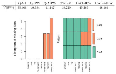
As done elsewhere in the literature, we compare two treatments of primary clinical interest at each stage: Perphenazine (coded -1) and Olanzapine (coded 1). The dataset consisting of 506 patients receiving these treatments , 46% of whom followed the entire course (i.e., they are complete cases), 34% dropped out after stage 1, and 20% dropped out after stage 2. The missingness pattern is shown in Figure 2.5. Item missingness was sparse (less than 2% of the observed data) and singly imputed using mean imputation.
p
Relativ
e V
alue
2 2 10 10 30 30 50 50
0.6
0.7
0.8
0.9
1.0
Missing rate = 35 %
IPW AIPW MI Missingness Model Correct
p
Relativ
e V
alue
2 2 10 10 30 30 50 50
0.3
0.4
0.5
0.6
0.7
0.8
0.9
1.0
Missing rate = 65 %
IPW AIPW MI Missingness Model Correct
p
Relativ
e V
alue
2 2 10 10 30 30 50 50
0.6
0.7
0.8
0.9
1.0
Missing rate = 35 %
IPW AIPW MI Missingness Model Correct
p
Relativ
e V
alue
2 2 10 10 30 30 50 50
0.3
0.4
0.5
0.6
0.7
0.8
0.9
1.0
Missing rate = 65 %
IPW AIPW MI Missingness Model Correct
p
Relativ
e V
alue
2 2 10 10 30 30 50 50
0.6
0.7
0.8
0.9
1.0
Missing rate = 35 %
IPW AIPW MI Missingness Model Misspecified
p
Relativ
e V
alue
2 2 10 10 30 30 50 50
0.3
0.4
0.5
0.6
0.7
0.8
0.9
1.0
Missing rate = 65 %
IPW AIPW MI Missingness Model Misspecified
p
Relativ
e V
alue
2 2 10 10 30 30 50 50
0.6
0.7
0.8
0.9
1.0
Missing rate = 35 %
IPW AIPW MI Missingness Model Misspecified
p
Relativ
e V
alue
2 2 10 10 30 30 50 50
0.3
0.4
0.5
0.6
0.7
0.8
0.9
1.0
Missing rate = 65 %
IPW AIPW MI Missingness Model Misspecified
Table 2.1 Cross-validated value estimates of the optimal regimes estimated using different methods.
Q-MI Q-IPW Q-AIPW OWL-MI OWL-IPW OWL-AIPW
b
V(πbopt) 35.406 40.684 41.147 48.220 49.366 48.164
Histogr
am of missing data
0.0 0.1 0.2 0.3 0.4 0.5 EXA
CER SEX TD
P ANSST O T .0 TREA T .1 P ANSST O T .1 TREA T .2 P ANSST O T .2 P atter n EXA
CER SEX TD
P ANSST O T .0 TREA T .1 P ANSST O T .1 TREA T .2 P ANSST O T .2 0.46 0.34 0.20
Figure 2.5 Missiningness pattern of CATIE study after cleaning.
decision rules for outcome weighted learning.
2.6
Discussion
CHAPTER
3
INTEGRATIVE ANALYSIS OF RANDOMIZED CLINICAL TRIALS
WITH REAL WORLD EVIDENCE STUDIES
3.1
Introduction
remains under-developed.
There is considerable interest in bridging the findings from a RCT to the target population. This problem has been termed as generalizability (Cole & Stuart, 2010; Stuart et al., 2011; Hernan & VanderWeele, 2011; Tipton, 2013; O’Muircheartaigh & Hedges, 2014; Stuart et al., 2015; Keiding & Louis, 2016; Buchanan et al., 2018), external validity (Rothwell, 2005) or transportability (Pearl & Bareinboim, 2011; Rudolph & Laan, 2017) in the statistics literature and has connections to the covariate shift problem in machine learning (Sugiyama & Kawanabe, 2012). Most of the existing methods rely on direct modeling of the sampling score, which is the sampling analog of the propensity score (Rosenbaum & Rubin, 1983a). The subsequent sampling score adjustments include inverse probability of sampling weighting (IPSW, Cole & Stuart, 2010; Buchanan et al., 2018), stratification (Tipton, 2013; O’Muircheartaigh & Hedges, 2014), and augmented IPSW (Dahabreh et al., 2018). There are two major drawbacks in the sampling score adjustment approaches. Firstly, they require correct model specification of the sampling score. The IPSW estimators are unstable or inconsistent if the sampling score is too extreme or misspecified. Secondly, they assume the RWE sample to be a simple random sample from the target population, and implicitly require either the population size or all the baseline information of the population to be available. For example, Dahabreh et al. (2018) set the target population to be all trial-eligible individuals and assumed that all population baseline covariates are known, which is rarely the case in practice.
To address the selection bias of the RCT sample, we estimate the sampling score weights directly by calibrating covariate balance between the RCT sample and the design-weighted RWE sample, in contrast to the dominant approaches that focus on predicting sample selection probabilities. Calibration weighting (CW) is widely used to integrate auxiliary information in survey sampling (Wu & Sitter, 2001; Chen et al., 2002; Kott, 2006; Chang & Kott, 2008; Kim et al., 2016), and causal inference, such as in Constrained Empirical Likelihood (Qin & Zhang, 2007), Entropy Balancing (Hainmueller, 2012), Inverse Probability Tilting (Graham et al., 2012), and Covariate Balance Propensity Score (Imai & Ratkovic, 2014; Fan et al., 2016). Chan et al. (2015) showed that estimating ATE by empirical balancing calibration weighting can achieve global efficiency. To the best of our knowledge, our paper is the first to use calibration in combining a RCT sample and a RWE sample to construct ATE estimators. We show that calibration weighting has several advantages in the data integration problem. First, its estimation does not require the population baseline covariates or the population size to be available, and it allows the RWE sample to be a general random sample, not necessarily a simple random sample, from the target population. Second, the weights are estimated directly from an optimization problem instead of inverting the estimated sampling probability, which requires careful monitoring to avoid extreme weights that result in highly variable estimates. Third, similar to Zhao & Percival (2017), we show that the calibration weighting estimators are doubly robust in the sense that the estimators are consistent if the parameterization for either the outcome or the sampling score model is correctly specified.
which allows flexible data-adaptive estimation of the nuisance functions while retaining usual root-nconsistency under mild regularity conditions.
The rest of this chapter is organized as follows. We formalize the causal framework and assumptions in Section 3.2. The CW estimators are introduced in Section 3.3. We provide the semiparametric efficiency bound and propose the augmented CW estimator in Section 3.4. The finite sample performances of the proposed estimators are evaluated and compared in simulations studies in Section 3.5. We apply the proposed methods to estimate the effect of adjuvant chemotherapy by integrating the RCT data for early-stage resected non–small-cell lung cancer with the real-world data from the National Cancer Database in Section 3.6. Section 3.7 concludes with future directions.
3.2
Basic setup
3.2.1 Notation: causal effect and two data sources
We let X be the p-dimensional vector of covariates; let A be the treatment assignment with two levels{0,1}, where 0 and 1 are the labels for control and active treatments, respectively; and let Y be the outcome of interest, which can be either continuous or binary. We use the potential outcomes framework (Neyman, 1923; Rubin, 1974) to formulate the causal problem. Under the Stable Unit Treatment Value Assumption (Rubin, 1980), for each level of treatmenta, we assume that each subject in the target population has a potential outcomeY(a), representing the outcome had the subject, possibly counterfactual, been given treatmenta. The conditional average treatment effect (CATE) is defined asτ(X) =E{Y(1)−Y(0)|X}. We are interested in estimating the population ATEτ0 =E{τ(X)}, where the expectation is taken with respect to the target population. If the outcome is binary, the ATE is referred to as the average causal risk differenceτ0 =P{Y(1) = 1} −P{Y(0) = 1}.
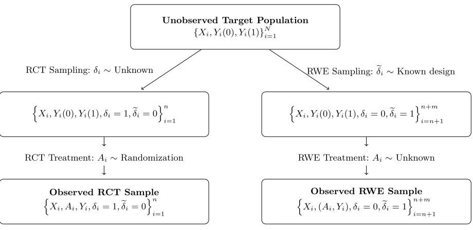
that compares the two treatments, and the other sample is from an observational RWE study that can be used to characterize the target population. The target population of size N consists of all patients with certain diseases to whom the new treatment is intended to be given. In practice, it is often difficult to identify the entire population, and the population size, N, is not necessarily known. Let δ = 1 denote RCT participation, and let eδ = 1 denote the RWE
study participation. The RWE sample is assumed to be a random sample drawn from the target population with a known sampling mechanism. Let d = 1/P(eδ = 1|X) be the design weight
in the RWE sample. For example, in health research, many cohort studies utilized stratified sampling to over-represent some subgroups. Suppose the population consists of Lstrata with sizes{N1, . . . , NL}, and suppose that the RWE study selects a fixed number of subjects nl from
theNl subjects in the lth stratum. Then, the design weight for subject j from thelth stratum
is dj =Nl/nl. We denote data from the RCT of size nto be {(Xi, Ai, Yi, δi = 1) :i= 1, ..., n};
the data from the RWE study of sizem to be eithern(Xj,δej = 1) : j =n+ 1, . . . , n+m o
if we only have covariate information, or n(Xj, Aj, Yj,δej = 1) : j=n+ 1, . . . , n+m
o
if treatment and outcome information are also available in the study. The data structure is demonstrated in Figure 3.1.
3.2.2 Identification assumptions
A fundamental problem in causal inference is that we can observe at most one of the potential outcomes for an individual subject. To identify the ATE from the observed data, we make the following assumptions throughout this chapter.
Assumption 1 (Consistency) The observed outcome is the potential outcome under the actual
received treatment: Y =AY(1) + (1−A)Y(0).
Unobserved Target Population
{Xi, Yi(0), Yi(1)}Ni=1
n
Xi, Yi(0), Yi(1), δi= 1,δei= 0
on
i=1
n
Xi, Yi(0), Yi(1), δi= 0,δei= 1
on+m
i=n+1 RCT Sampling:δi∼Unknown RWE Sampling:eδi∼Known design
RCT Treatment:Ai∼Randomization RWE Treatment:Ai∼Unknown
Observed RCT Sample n
Xi, Ai, Yi, δi= 1,eδi= 0
on
i=1
Observed RWE Sample n
Xi,(Ai, Yi), δi= 0,eδi= 1
on+m
i=n+1
Figure 3.1 Demonstration of the sampling and treatment assignment regimes for the RCT and RWE samples within the target population.
Assumption 2 (i) holds for the RCT by default. Assumption 2 (ii) requires that the CATE function is transportable from the RCT to the target population. This assumption relaxes the ignorability assumption on trial participation (Stuart et al., 2011; Buchanan et al., 2018), i.e., {Y(0), Y(1)}⊥δ |X, and the mean exchangeability assumption over treatment assignment and trial participation (Dahabreh et al., 2018), i.e.E{Y(a)|X, δ = 1, A=a}=E{Y(a)|X, δ = 1} as well asE{Y(a)|X, δ= 1}=E{Y(a)|X} fora= 0,1.
Moreover, we require adequate overlap of the covariate distribution between the trial sample and the target population, and also the treatment groups over the trial sample, formalized by the following assumption. Define the sampling score asπδ(X) =P(δ= 1|X) .
Assumption 3 (Positivity) There exists a constant c such that with probability 1, πδ(X)≥
Under Assumptions 1–3, the ATE satisfies
τ0 = E{τ(X)}=E[E{Y(1)−Y(0)|X, δ= 1}]
= E
δ πδ(X)
{E(Y |X, A= 1, δ= 1)−E(Y |X, A= 0, δ= 1)}
= Eheδd{E(Y |X, A= 1, δ= 1)−E(Y |X, A= 0, δ= 1)} i
,
and thus is identifiable.
3.2.3 Existing estimation methods
Because the RCT assigns treatments randomly to the participants,τ(X) is identifiable and can be estimated by standard estimators solely from the RCT. However, the covariate distribution of the RCT samplef(X |δ= 1) is different from that of the target population f(X) in general; therefore,E{τ(X)|δ = 1} is different from τ0, and the ATE estimator using trial data only is biased of τ0 generally.
A widely-used approach is the IPSW estimator that predicts the sampling score πδ(X)
and uses the inverse of the estimated sampling score to account for the shift of the covariate distribution from the RCT sample to the target population. Specifically, most of the empirical literature assumes thatπδ(X) follows a logistic regression modelπδ(X;η) and can be estimated
by πδ(X;ηb). The IPSW estimator of the ATE is
ˆ
τIPSW =
Pn
i=1πδ(Xi;ηb)
−1A
iYi
Pn
i=1πδ(Xi;ηb)
−1A
i
−
Pn
i=1πδ(Xi;ηb)
−1(1−A
i)Yi
Pn
i=1πδ(Xi;ηb)
−1(1−A
i)
. (3.1)
3.3
Calibration weighting estimators
We propose to use calibration originated in survey sampling to eliminate the selection bias in the trial-based ATE estimator. The calibration weighting approach is similar to the idea of entropy balancing weights introduced by Hainmueller (2012). We calibrate subjects in the RCT sample so that after calibration, the covariate distribution of the RCT sample empirically matches the target population. Our insight is based on the observation that for any vector-valued function
g(X),
E
δ πδ(X)
g(X)
=Eneδdg(X) o
=E{g(X)}.
Here,g(X) contains the covariate functions to be calibrated, which could be moment functions of the original covariateX or any sensible transformations of X.
To this end, we assign a weight qi to each subject iin the RCT sample so that N
X
i=1
δiqig(Xi) =ge, (3.2)
where eg=
PN
i=1δeidig(Xi)/
PN
i=1δeidi is a design-weighted estimate ofE{g(X)} from the RWE
sample. Constraint (3.2) is referred to as the balancing constraint, and weights Q ={qi :δi = 1}
are the calibration weights. The balancing constraint calibrates the covariate distribution of the RCT sample to the target population in terms ofg(X). The choice of g(X) is important for both bias and variance considerations, which we will discuss in Section 3.4.2.
We estimate Q by solving the following optimization problem:
min Q
n X
i=1
qilogqi, (3.3)
subject to qi ≥0, for alli;Pni=1qi= 1, and the balancing constraint (3.2).
this criteria ensures that the empirical distribution of calibration weights are not too far away from the uniform, such that it minimizes the variability due to heterogeneous weights. This optimization problem can be solved using convex optimization with Lagrange multiplier. By introducing Lagrange multiplierλ, the objective function becomes
L(λ,Q) =
n X
i=1
qilogqi−λ>
( n
X
i=1
qig(Xi)−eg )
. (3.4)
Thus by minimizing (3.4), the estimated weights are
b
qi=q(Xi;λb) =
exp
n b
λ>g(Xi) o
Pn
i=1exp
n b
λ>g(Xi)
o,
and λb solves the equation
U(λ) =
n X
i=1
expnλ>g(Xi) o
{g(Xi)−ge}= 0, (3.5)
which is the dual problem to the optimization problem (3.3).
There are two general types of weighted estimators for population means, namely the Horvitz-Thompson estimator (HT, Horvitz & Horvitz-Thompson, 1952) and the Hajek estimator (H´ajek, 1971). We propose both estimators with the superscript 0 for the HT estimator and the superscript 1 for the Hajek estimator. Let πAi=P(Ai = 1|Xi, δi = 1) be the treatment propensity score for
subject i. For RCTs, it is common that the propensity score is known with πAi = 0.5, for all
i= 1, . . . , n.
Based on the calibration weights, we propose the HT CW estimator
ˆ τCW0=
n X i=1 b qi
AiYi
πAi
− (1−Ai)Yi 1−πAi
and the Hajek CW estimator
ˆ τCW1=
n X
i=1
b
qi
AiYi
Pn
i=1Aiqbi
−Pn(1−Ai)Yi
i=1(1−Ai)qbi
. (3.7)
To investigate the properties of the proposed CW estimators, we impose the following regularity conditions on the sampling designs for both the RWE and the RCT samples.
Assumption 4 Let µg0 =E{g(X)}. The design weighted estimator µgb =N
−1PN
i=1δeidig(Xi) satisfiesV(µbg) =O(m−1), and{V(µbg)}
−1/2(
b
µg−µg0)→N(0,1)in distribution, as m→ ∞.
Assumption 5 The sampling score of RCT participation follows a loglinear model, i.e.πδ(X) =
exp{η>0g(X)} for some η0.
Note that if the sampling score follows a logistic regression modelπδ(X;η) = exp{η>g(X)}/[1+
exp{η>g(X)}] and the sampling fraction of the RCT is small, the loglinear model in Assumption 5 is close to the logistic regression model. Our simulation studies demonstrate that the proposed estimators perform well under a logistic regression model.
In addition, in the estimation of calibration weights we only require specifying g(X). Thus, CW evades explicitly modeling either the sampling score model or the outcome mean models. Under Assumption 5, we show that there is a direct correspondence between calibration weight q(Xi;λb) and the estimated sampling scoreπδ(Xi;ηb), i.e.q(Xi;λb) ={N πδ(Xi;ηb)}
−1+o
p(N−1);
see the proof of Theorem 3 in the Appendix.
The following assumption is on the linearity of the CATE ing(X).
Assumption 6 τ(X) =γ0>g(X).