DOI: http://dx.doi.org/10.26483/ijarcs.v8i9.4940
Volume 8, No. 9, November-December 2017
International Journal of Advanced Research in Computer Science
RESEARCH PAPER
Available Online at www.ijarcs.info
ISSN No. 0976-5697
CLASSIFICATION OF SPARQL QUERIES INTO EQUIVALENCE CLASSES OF
RELEVANT QUERIES
Theodore Andronikos
Department of Informatics Ionian University
Corfu, Greece
Abstract: This paper is inspired by ideas from the field of theoretical Mathematics, used for the partitioning of abstract spaces into equivalence classes, and applies analogous concepts in order to propose a classification of SPARQL queries into equivalence classes. The novel concepts of relevant queries and covering query are introduced in a manner appropriate for the study of SPARQL queries. These new definitions shed new light on the relations among SPARQL queries. They enable the formal identification of similar queries and this leads to the partition of SPARQL queries into equivalence classes of relevant queries. This work also discusses how the covering query relating two or more relevant queries can be useful from the perspective of computational cost when evaluating composite queries composed of simpler relevant queries. Hence, the introduction of the concept of relevance between queries provides not only obvious theoretical advantages, but also concrete practical ones, which in many cases have the potential to lower the computational cost of query evaluation.
Keywords: RDF graph, SPARQL query, relevant query, classification, equivalence class
1.INTRODUCTION
Today one of the most important areas of research is undoubtedly the Semantic Web. During the last decade, Semantic Web, combined with a spectrum of related technologies, e.g., Linked Open Data [1], has forever transformed the way we perceive the World Wide Web. One of the key reasons for the success of Semantic Web is the fact that it is based on standards. The Resource Description Framework (RDF) and SPARQL are probably the two most important standards of the Semantic Web.
The Resource Description Framework is used to store data in the form of a directed graph [2]. The contents of the directed graph are viewed as triples (subject, predicate, object), where the subject is related to the object through the predicate. SPARQL [3] is the de facto standard language that is used for querying RDF datasets. Of particular importance from our viewpoint is the class of Regular Path Queries (RPQ for short). These are SPARQL queries that concern pairs of nodes of the RDF graph. An underlying path consisting of directed edges of the RDF graph begins from the first node and terminates at the second node. This path satisfies certain properties and these properties are formulated in terms of simple regular expressions that are suitable for this purpose.
In this context, the so called “transitive” predicates play a particularly important role. A predicate R, which can conveniently be viewed as a label of one or more directed edges of the RDF graph, is called transitive if one can validly infer the triple that (a, R, c) from the existence of the two triples (a, R, b) and (b, R, c) in the RDF dataset.
SPARQL queries taking advantage and utilizing transitive predicates are the most suitable examples for demonstrating the concept of “relevant” queries, which is the main theme of this paper. This work is inspired by theoretical ideas from the field of Mathematics which are used in order to access the similarity between abstract mathematical notions. We investigate how these ideas can be infused in the
context of SPARQL queries so as to provide a theoretical partition of the set of SPARQL queries into equivalence classes, where each class contains “relevant” queries, that is queries that are connected in a precise formal way.
Contribution. The main contribution of this work lies in its novelty. This paper advocates the use of mathematical notions for the classification of SPARQL queries into equivalence classes. Mathematical ideas have always been used in a fruitful way to tackle concrete computational problems. Following this line of thought, this work proposes the use of abstract mathematical concepts as a tool for the classification and subsequent evaluation of SPARQL queries. The idea of relevant SPARQL queries, which is introduced here, has far-reaching ramifications because it reveals hidden connections between queries. These connections, apart from being of interest in their own right, can also be used to improve the computational cost of evaluating those composite SPARQL queries that are comprised of relevant queries. In such composite queries, which are often encountered in practice, a covering query, that is a query that establishes the formal connection among the relevant queries, can be used instead of the individual relevant queries. The use of a covering query is advantageous because it will enable the evaluation of the composite query in a more efficient manner, requiring less computational time.
The paper is organized as follows: Section 2 contains references to other related works, Section 3 presents the definitions and the notation used in this work, Section 4 lists and analyzes the main results, and, finally, Section 5 summarizes conclusions and suggests some possible ideas for future work.
2.RELATEDWORK
query is not a SPARQL query applicable to a RDF dataset, but just a keyword based query, typically submitted by the user when searching for some information in the internet. The present paper focuses on SPARQL queries and establishes a type of similarity among such queries based upon a rigorous definition. To avoid any potential confusion, we shall henceforth use the characterization “relevant” in our study of SPARQL queries. In the rest of this section we briefly mention a few other works that are related to the present article in the sense that they focus on SPARQL and RDF graphs from a theoretical viewpoint.
In [6] Schmidt et al. study equivalences in the context of SPARQL algebra. The main theme of their work is the classification of SPARQL fragments in complexity classes. They extensively use SPARQL set algebra and study both set and bag semantics. Our work is different from theirs in that we give a totally different and completely new definition for the equivalence of SPARQL queries, introducing at the same time the novel concept of covering query, and we also avoid the use SPARQL algebra.
Zhang et al. [7] proposed an extension of navigational path queries using elements from the theory of context-free languages. Since context-free constructs are more expressive than regular expressions, this approach enhances the expressive power of SPARQL queries. The resulting language is named cfSPARQL and, as the name suggests, endows standard SPARQL with context-free grammars. cfSPARQL enables the user to formulate more powerful and complex queries that SPARQL. The authors claim that the increased expressive power does not come up with an increased computational cost, i.e., in most practical examples query evaluation in cfSPARQL remains efficient.
An important theoretical work by Sistla et al. [8] demonstrated the relationship of database queries with finite automata. In [8] the authors developed a technique by which database queries, e.g., nearest neighbor queries, are expressed using an automata-theoretic approach. Ideas and methods from the theory of finite automata motivated Wang et al. in [9] to devise an algorithm suitable for evaluating RDF queries. They also presented experimental results that confirm that the methodology they propose is capable of handling efficiently certain categories of regular path queries on large scale RDF graphs.
Another theoretical work that investigated the correlation of queries on RDF datasets to certain types of finite automata appeared in [10]. There the emphasis was on the practically infinite nature of Linked Data apothecaries, which is a reasonable abstraction if one takes into account their ever increasing size. This line of thought was further pursued in [11], where a connection between SPARQL queries involving transitive predicates and ω-regular languages, i.e., the analog of regular languages in case of infinite words, and finite automata accepting infinite inputs is established. Tools and techniques from the theory of probabilistic automata can also be used when dealing with data characterized by a certain degree of uncertainty, e.g., biomedical data, as was demonstrated in [12].
All the previous references serve to indicate that ideas and methods originating from theoretical disciplines can be successfully adopted to more concrete and practical environments, such as evaluation of SPARQL queries. It is this point of view that characterizes this paper, where the inspiration comes from the field of mathematics and leads to
the introduction of novel notion like relevant queries and covering query.
3.DEFINITIONSANDNOTATION
SPARQL queries return information stored in a RDF graph. The underlying syntax is rather user-friendly and enables the user to retrieve data that match a certain pattern. In this work we shall use the notation designated in the following definition for the answer set returned by a query q when applied on the dataset D. The examples used to demonstrate the concept of relevant queries will rely on the use of so called transitive predicates and will take advantage of the new navigational capabilities of SPARQL 1.1 [2].
Definition 1. Let q(x1, …, xn) be a SPARQL query involving the n projection variables ?x1, …, ?xn in the SELECT clause of the query, and let D be a RDF dataset. The result of applying q(x1, …, xn) on D will be called the answer set of q over D and will be denoted by q(x1, …, xn)[D].
Consider a simple SPARQL query Q(x1, x2) like the one shown in Figure 1a.
SELECT ?x1 ?x2 WHERE {
?x1 IsConnectedTo ?x2 . }
Figure 1a. The above SPARQL query lists the ordered pairs (x1, x2) such that there is an edge from x1 to x2 labeled by the predicate IsConnectedTo.
SELECT ?x1 WHERE {
?x1 IsConnectedTo destination . }
Figure 1b. The above SPARQL query outputs the nodes x1 connected to destination by the predicate IsConnectedTo.
SELECT ?x2 WHERE {
source IsConnectedTo ?x2 . }
Figure 1c. The above SPARQL query returns the nodes x2 for which there is an edge from the node source to x2 labeled by the predicate IsConnectedTo.
be convenient to introduce the following notation to describe such substitutions of variables by constants.
Definition 2. Let q(x1, …, xn) be a SPARQL query involving the n projection variables ?x1, …, ?xn in the SELECT clause of the query. We write q(x1, …, xn){xi1|c1, …, xim|cm} to denote the query q´ arising from q, if all the m projection variables ?xi1, …, ?xim are removed from the SELECT clause of q(x1, …, xn) and all remaining occurrences of ?xi1, …, ?xim are replaced by the m constants c1, …, cm, respectively. Obviously, m ≤ n.
With the above notation, the queries Q´(x1) and Q´´(x2), depicted in Figure 1b and Figure 1c, respectively, can be written as Q(x1, x2){x2|destination} and Q(x1, x2){x1|source}, which immediately reveals that are special instances of the more general query Q(x1, x2) of Figure 1a. In the sequel, we will often refer to such an action as the application of a substitution to a given query, e.g., applying the substitution {x2|destination} to Q(x1, x2), will give rise to the Q´(x1).
Remark 1. If a query q´(y1, …, yn) containing exactly n projection variables, results from the query q(x1, …, xn), also containing exactly n projection variables, by renaming all occurrences of x1, …, xn to y1, …, y, respectively, then the queries q and q´ will be considered identical. In other words, consistent renaming of the projection variables in a query leaves the query unchanged and so q(x1, …, xn) and q´(y1, …, yn) are in fact the same query.
Consider two SPARQL queries q1 and q2 and let us further assume that both queries involve n projection variables. We call q1 and q2 relevant if they can be related by another query Q that utilizes at least n variables. Formally, the following definition captures the notion of relevance between queries.
Definition 3. Let q1(x1, …, xn) and q2(x1, …, xn) be two queries with exactly n projection variables. The query q1(x1, …, xn) is relevant to the query q2(x1, …, xn), if there exists a query Q(x1, …, xn, xn+1, …, xn+m), where m≥ 0, such that for every RDF dataset D:
(1) q1(x1, …, xn)[D] = Q1(xi1, …, xin)[D], where Q1(xi1, …, xin) = Q(x1, …, xn, xn+1, …, xn+m){xj1|c1, …, xjm|cm}, and
(2) q2(x1, …, xn)[D] = Q2(xk1, …, xkn)[D], where Q2(xk1, …, xkn) = Q(x1, …, xn, xn+1, …, xn+m){xr1|c1, …, xrm|cm}.
The query Q(x1, …, xn, xn+1, …, xn+m) is a covering query for both q1(x1, …, xn) and q2(x1, …, xn).
We write q1 ~ q2 to denote that q1 and q2 are relevant.
Some clarifications are perhaps necessary in order to better understand the above definition.
• First, we emphasize that the covering query Q involves n+m, where m ≥ 0, projection variables, whereas each of the two relevant queries q1 and q2 involve exactly n projection variables.
• In writing Q1(xi1, …, xin) and Q2(xk1, …, xkn), the meaning is that both Q1(xi1, …, xin) and Q2(xk1, …, xkn) result from the covering query Q(x1, …, xn, xn+1, …, xn+m) by substituting the m remaining projection variables by m constants. In the first case the m constants are c1, …, cm and in the second case the m constants are d1, …, dm.
• The resulting query Q1(xi1, …, xin) involves the n projection variables xi1, …, xin. Likewise, Q2(xk1, …, xkn) involves the n projection variables xk1, …, xkn. These n projection variables are in general different and are also different from the n initial variables x1, …, xn of the covering query Q.
• The answer sets Q1(xi1, …, xin)[D] and Q2(xk1, …, xkn)[D] are sets of n tuples, as required to achieve the equality with the answer sets q1(x1, …, xn)[D] and q2(x1, …, xn)[D], respectively.
• The constants c1, …, cm and d1, …, dm correspond to URIs appearing in D and will also in general be different.
The following example will hopefully serve as a useful introduction to the notion of relevant queries.
Example 1. Consider the SPARQL query q1 shown in Figure 2a. This query when applied to a RDF graph that contains the transitive predicate P will return all those nodes that are connected to the node destination through one or more edges labeled by the same transitive predicate P.
Let us emphasize that in this query we regard predicate P as transitive in sense that if (a, P, b) and (b, P, c) are two triples stored in the RDF dataset, then, on a semantic level, we may infer that (a, P, c). Moreover, q1 utilizes the capabilities of SPARQL 1.1 [3], the syntax of which enables us to define and process path properties. The special symbol + is interpreted as asserting the existence of one or more edges labeled by the transitive predicate P.
SELECT ?x WHERE {
?x P+ destination . }
Figure 2a. The SPARQL query q1 lists the nodes that are connected to the node destination through one or more edges labeled by the transitive predicate P.
SELECT ?x1 WHERE {
source P+ ?x . }
Figure 2b. The SPARQL query q2 outputs the nodes that are connected to the initial node source via one or more edges labeled by the transitive predicate P.
SELECT ?x1 ?x2 WHERE {
?x1 P+ ?x2 . }
Figure 2c. The SPARQL query Q returns the pairs of nodes that are connected by a path consisting of one or more edges labeled by the transitive predicate P.
The two queries q1 and q2 can be regarded as similar in view of the fact that both return nodes that form a path of length at least one, which is labeled by the same predicate (in our case the transitive predicate P). The difference is that in the first case the path terminates at a specific node, namely the node destination, whereas in the second case the path begins at a specific node (the node source).
It should therefore come as no surprise that there is another SPARQL query Q, the one depicted in Figure 2c, which is closely related to both queries q1 and q2, or, from another viewpoint, that relates explicitly q1 and q2. It is rather straightforward to see that Q returns all the ordered pairs (x1, x2) such that there exists a path of length at least one from x1
to x2 labeled by the transitive predicate P. This of course
means that all nodes in q1(x)[D] appear as the first element of an ordered pair of Q(x1, x2)[D] and symmetrically all elements of q2(x)[D] appear as the second element of an ordered pair of Q(x1, x2)[D]. Moreover, by substituting the constant destination for all occurrences of the projection variable x2 in Q, the resulting query Q1(x1) = Q(x1, x2){x2|destination} is none other than the query q1(x). Symmetrically, by substituting the constant source for all occurrences of the projection variable x1 in Q, the resulting query Q2(x2) = Q(x1, x2){x1|source} becomes precisely the query q2(x). Therefore, according to Definition 3, Q(x1, x2) is indeed a covering query for q1(x) and q2(x) because q1(x)[D] = Q1(x1)[D] and q2(x)[D] = Q2(x2)[D]. ▲
The previous Example 1 is quite simple, but the following example will demonstrate that relevant queries can be significantly more complex. From now for brevity we shall adopt the following terminology: a path consisting of edges labeled by the same transitive predicate P will simply be called a P-path. Whenever we want to express the fact that x is the first node and y is the terminal node of such a P-path we shall write x⇒Py.
SELECT ?x1 ?x2 WHERE {
?x1 P+ ?x2 . ?x2 R+ destination . }
Figure 3a. The SPARQL query q1 lists the ordered pairs (x1, x2) such that x1 is connected to x2 via a P -path and x2 is connected to the node destination through an R-path. Both paths are of length at least one.
SELECT ?x1 ?x3 WHERE {
?x1 P+ intermediate . intermediate R+ ?x3 . }
Figure 3b. The SPARQL query q2 outputs the ordered pairs (x1, x3) such that x1 is connected to the node intermediate via a P-path and intermediate is connected to x3 through an R-path. Both paths are of length at least one.
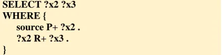
SELECT ?x2 ?x3 WHERE {
source P+ ?x2 . ?x2 R+ ?x3 . }
Figure 3c. The SPARQL query q3 returns the ordered pairs (x2, x3) such that there exists a P-path from source to x2, and x2, is connected to x3 through an R -path. Both paths are of length at least one.
SELECT ?x1 ?x2 ?x3 WHERE {
?x1 P+ ?x2 . ?x2 R+ ?x3 . }
Figure 3d. The above SPARQL query lists the ordered triples (x1, x2, x3) such that there exists a P -path from x1 to x2, and an R- from x2 to x3. Both paths are of length at least one.
Example 2. In this example, we begin by considering the SPARQL query q1 shown in Figure 3a. This query contains not just one but two transitive predicates: P and R and involves two variables x1 and x2. When applied on a suitable RDF graph it will return all those ordered pairs (x1, x2) such that x1 is connected to x2 via a P-path of length at least one and x2 is connected to the node destination through an R-path of length at least one.
The SPARQL query q2 shown in Figure 3b will list all ordered pairs (x1, x3) such that x1 is connected to the node intermediate via a P-path of length at least one and, in turn, intermediate is connected to x3 through an R-path of length at least one.
A similar examination of the query q3 of Figure 3c, shows that q3 outputs all ordered pairs (x2, x3) such that there exists a P-path of length at least one from the node source to
x2 and there exists also an R-path of length at least one from
the x2 to x3.
The relevance of queries q1, q2 and q3 is rather obvious. All three of them return nodes that form precisely two paths: a P-path followed by an R-path. The difference among the three queries is in the specifics. For the q1 query the R-path must terminate at the node destination, for the q2 query the P-path must terminate at the node intermediate and the R -path must begin at the node intermediate, and for the q3 query the P-path must begin at the node source.
The SPARQL query Q(x1, x2, x3) depicted in Figure 3d is the covering query for q1, q2 and q3. Q(x1, x2, x3) is more complex that q1, q2 and q3. While each of q1, q2 and q3 involve two projection variables, Q(x1, x2, x3) involves three projection variables. As a result Q returns ordered triples (x1, x2, x3); in each such triple x1 is connected to x2 via a P-path
and x2 is connected to x3 through an R-path. More formally,
by evaluating Q to the dataset D, we get the answer set Q(x1, x2, x3)[D] = {(x1, x2, x3) : x1⇒Px2 and x2⇒Rx3}.
[image:4.595.327.552.56.112.2]occurrences of the projection variable ?x2 in Q, the resulting query Q2(x1, x3) = Q(x1, x2, x3){x2|intermediate} is just the query q2(x1, x3). Finally, by substituting the constant source for all occurrences of the projection variable ?x1 in Q, the resulting query Q3(x2, x3) = Q(x1, x2, x3){x1|source} is simply the query q3(x2, x3).
Obviously, Q(x1, x2, x3) is a covering query for q1, q2 and q3, since q1(x1, x2)[D] = Q1(x1, x2)[D], q2(x1, x3)[D] = Q2(x1, x3)[D], and q3(x2, x3)[D] = Q3(x2, x3)[D]. ▲
4. FUNDAMENTAL PROPERTIES OF RELEVANT QUERIES
From a theoretical point of view, the relevance relation between queries satisfies certain important properties. This is expressed in the next proposition.
Proposition 1. The relevance relation ~ between queries is an equivalence relation.
Proof.
We must check that the relation ~ satisfies the following three properties that characterize equivalence.
(1) The reflexive property requires to show that for every query q(x1, …, xn), it holds that q(x1, …, xn) ~ q(x1, …, xn). This is rather trivial because we can take the query q(x1, …,
xn) itself as the covering query.
(2) Suppose now that q1(x1, …, xn) ~ q2(x1, …, xn). We have to prove the symmetric property, i.e., that also q2(x1, …, xn) ~ q1(x1, …, xn). The fact that q1 and q2 are relevant implies that there exists a covering query Q(x1, …, xn, xn+1, …, xn+m), where m≥ 0, and two substitutions θ1 and θ2, which are, in general, different, for m of the projection variables that satisfy the requirements of Definition 3. In particular, if Q(x1, …, xn, xn+1, …, xn+m) θ1 = Q1(xi1, …, xin) and Q(x1, …, xn, xn+1, …, xn+m) θ2 = Q2(xk1, …, xkn), then q1(x1, …, xn)[D] = Q1(xi1, …, xin)[D] and q2(x1, …, xn)[D] = Q2(xk1, …, xkn)[D] for every RDF database D. This immediately gives that q2(x1,
…, xn) ~ q1(x1, …, xn) via the same covering query Q(x1, …,
xn, xn+1, …, xn+m).
(3) Finally, suppose that q1(x1, …, xn) ~ q2(x1, …, xn) and q2(x1, …, xn) ~ q3(x1, …, xn). To establish the transitive property, we must that also q1(x1, …, xn) ~ q3(x1, …, xn). The two hypotheses imply the existence of two covering queries Q1(x1, …, xn, xn+1, …, xn+m) and Q2(x1, …, xn, xn+1, …, xn+m´),
and four substitutions θ1, θ2, θ3, θ4, such that q1(x1, …, xn)[D] = U1(xi1, …, xin)[D], q2(x1, …, xn)[D] = U2(xk1, …, xkn)[D], where U1(xi1, …, xin) = Q1(x1, …, xn, xn+1, …, xn+m) θ1, U2(xk1, …, xkn) = Q1(x1, …, xn, xn+1, …, xn+m) θ2, and q2(x1, …, xn)[D] = V1(xr1, …, xrn)[D], q3(x1, …, xn)[D] = V2(xt1, …, xtn)[D], where V1(xr1, …, xrn) = Q2(x1, …, xn, xn+1, …, xn+m´) θ3, V2(xt1, …, xtn) = Q2(x1, …, xn, xn+1, …, xn+m´) θ4. We construct a new
query Q that contains as subqueries the queries Q1 and Q2. We may assume that Q1 and Q2 have no variable names in common. Even if this is not the case, we may rename the projection variables of Q2 to ensure that the all variables are distinct. This renaming does not change the semantics of Q2 (recall Remark 1) and the resulting query is the semantically equivalent to Q2. The projection variables of Q are comprised of the projection variables of Q1, the projection variables of Q2 (after they have been renamed, if necessary), and a new variable, which we call ?choice. Moreover, we construct a new substitution θ1´ by augmenting θ1 with substitutions of the projection variables y1, …, yn, yn+1, …, yn+m´ of Q2 by
constants d1, …, dn, dn+1, …, dn+m´, and the substitution of
choice by a string constant, e.g., “first”. The resulting substitution θ1´ is θ1∪{y1|d1, …, yn|dn, yn+1|dn+1, ..., yn+m´|dn+m´, choice|“first”}. The subquery Q1 is also augmented with a FILTER statement testing whether ?choice is equal to the string constant used in θ1´, e.g., “first”. This guarantees that the augmented subquery returns exactly the same answer set as θ1´ when θ1´ is used and nothing whenever a different substitution for ?choice is used. Symmetrically, starting from θ4, we construct the new substitution θ4´ = θ4∪{x1|c1, …, xn|cn, xn+1|cn+1, ..., xn+m|cn+m, choice|“second”}. Likewise, Q2 is also augmented with a FILTER statement involving ?choice that passes the results only when the substitution θ4´ is used.
Therefore, by the above construction, we conclude that q1(x1, …, xn)[D] = W1(xi1, …, xin)[D] and q3(y1, …, yn)[D] = W2(xt1, …, xtn)[D], where W1(xi1, …, xin) = Q(x1, …, xn, xn+1, …, xn+m, y1, …, yn, yn+1, …, yn+m´, choice) θ1´ and W2(xt1, …, xtn) = Q(x1, …, xn, xn+1, …, xn+m, y1, …, yn, yn+1, …, yn+m´,
choice) θ4´. This proves that Q is a covering query for q1 and q3 and, thus, q1 ~ q3.
Example 3. This example will shed some light on the construction we used in Proposition 1 in order to establish the transitive property of the ~ relation.
The queries q1 and q2 shown in Figure 4a are relevant and the covering query Q1 that establishes this fact is also shown in Figure 4a. The two substitutions that, when applied to Q1, establish the relation q1 ~ q2 are {x3|IsSolid} and {x2|metallicObject} for q1 and q2, respectively.
The queries q2 and q3, shown in Figure 4b, are also relevant. A covering query for q2 and q3 is the query Q2 also depicted in Figure 4b. The two substitutions that establish that q2 ~ q3 are {x2|metallicObject} for q2 and {x1|bolt} for q3, respectively.
The algorithm described in Proposition 1 results in the construction of the query Q shown in Figure 4c. To avoid any clash of names and any possible ambiguity, the projection variables x1, x2, x3 of Q2 are consistently renamed to y1, y2, y3. This ensures that there are no variable names in common between Q1 and Q2. Moreover, this renaming does not change the semantics of Q2 (recall Remark 1), meaning that the resulting query is the same as Q2.
SELECT ?x1 ?x2 WHERE {
?x1 IsInstanceOf ?x2. ?x2 HasProperty IsSolid. }
(q1)
SELECT ?x1 ?x3 WHERE {
?x1 IsInstanceOf metallicObject. metallicObject HasProperty ?x3. }
(q2)
SELECT ?x1 ?x2 ?x3 WHERE {
?x1 IsInstanceOf ?x2. ?x2 HasProperty ?x3.
}
Figure 4a. The first SPARQL query q1 above is relevant to the second query q2. The covering query that establishes that q1 ~ q2 is the query Q1.
SELECT ?x1 ?x3 WHERE {
?x1 IsInstanceOf metallicObject. metallicObject HasProperty ?x3. }
(q2)
SELECT ?x2 ?x3 WHERE {
bolt IsInstanceOf ?x2. ?x2 HasProperty ?x3. }
(q3)
SELECT ?x1 ?x2 ?x3 WHERE {
?x1 IsInstanceOf ?x2. ?x2 HasProperty ?x3. }
(Q2)
Figure 4b. Similarly, q2 ~ q3 and Q2 is a covering query for q2 and q3.
SELECT ?x1 ?x2 ?x3 ?y1 ?y2 ?y3 ?choice WHERE {
{
SELECT ?x1 ?x2 ?x3 WHERE {
?x1 IsInstanceOf ?x2 . ?x2 HasProperty ?x3 . FILTER ( ?choice = “first” ) }
} {
SELECT ?y1 ?y2 ?y3 WHERE {
?y1 IsInstanceOf ?y2 . ?y2 HasProperty ?y3 .
FILTER ( ?choice = “second” ) }
} }
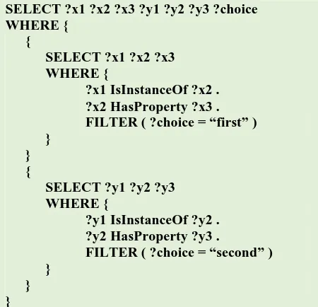
Figure 4c. The above query Q is a covering query for q1 and q3.
Hence, the variables appearing in the SELECT clause of Q are the variables x1, x2, x3 of Q1, the variables y1, y2, y3 of Q2, and a new projection variable ?choice, which will be used to filter the results returned by the two subqueries.
SELECT ?x1 ?x2 WHERE {
{
SELECT ?x1 ?x2 WHERE {
?x1 IsInstanceOf ?x2 . ?x2 HasProperty IsSolid . FILTER ( “first” = “first” ) }
} {
SELECT WHERE {
d1 IsInstanceOf d2 . d2 HasProperty d3 .
FILTER ( “first” = “second” ) }
[image:6.595.47.270.140.336.2]} }
Figure 5a. The above SPARQL query W1(x1, x2) arises from the query Q(x1, x2, x3, y1, y2, y3, choice) of Figure 4c with the substitution {x3|IsSolid, y1|d1, y2|d2, y3|d3, choice|“first”}, where d1, d2, d3 are arbitrary constants. The FILTER statements in the two subqueries guarantee that W1 returns all ordered pairs (x1, x2) from subquery Q1 but none from subquery Q2.
SELECT ?y2 ?y3 WHERE {
{
SELECT WHERE {
c1 IsInstanceOf c2 . c2 HasProperty c3 .
FILTER ( “second” = “first” ) }
} {
SELECT ?y2 ?y3 WHERE {
bolt IsInstanceOf ?y2 . ?y2 HasProperty ?y3 .
FILTER ( “second” = “second” ) }
[image:6.595.326.550.316.534.2]} }
Figure 5b. The above query W2(y2, y3) arises from the query Q(x1, x2, x3, y1, y2, y3, choice) of Figure 4c with the substitution {x1|c1, x2|c2, x3|c3, y1|bolt, choice|“second”}, where c1, c2, c3 are arbitrary constants. The FILTER statements in the two subqueries guarantee that W2 returns all ordered pairs (y2, y3) from subquery Q2 but none from Q1.
Applying the substitution {x3|IsSolid, y1|d1, y2|d2, y3|d3, choice|“first”}, where d1, d2, d3 are arbitrary constants, to the query Q(x1, x2, x3, y1, y2, y3, choice), results in the query W1(x1, x2) depicted in Figure 5a. In view of the fact that the second FILTER statement will exclude everything, while the first FILTER statement will allow everything, we conclude that W1(x1, x2) is equivalent to Q1{x3|IsSolid}. Therefore, W1(x1, x2)[D] = q1(x1, x2)[D].
[image:6.595.46.271.381.598.2] [image:6.595.45.272.715.786.2]Q(x1, x2, x3, y1, y2, y3, choice). In this case, the first FILTER statement will exclude everything, while the second FILTER statement will allow everything. This implies that W2(y2, y3) is equivalent to Q2{y1|bolt}, and, therefore, W2(y2, y3)[D] = q3(y2, y3)[D]. This concludes the proof that Q is a covering query for q1 and q3 and, thus, q1 ~ q3. ▲
The construction the query Q that establishes the transitivity of the relevance relation ~ was somewhat artificial and mechanical. It serves only to complete the proof. Clearly, there is a high degree of redundancy in Q, which is not at all optimized. In most practical cases, things will be much easier. For instance, in Example 3, query Q1 alone suffices to establish that q1 ~ q3. This is achieved with the substitutions {x3|IsSolid} and {x1|bolt} for q1 and q3, respectively.
Proposition 1 is important because it means that the set of SPARQL queries is partitioned into equivalence classes, and each SPARQL query q belongs to one such class.
Definition 4. Let q be a SPARQL query. The equivalence class to which q belongs is denoted by [q]. Alternatively, we say that q is a representative of the class [q].
Having established this theoretical classification of SPARQL queries into equivalence classes, let us turn our attention into possible ways to take advantage of this situation for practical purposes.
Consider a scenario where we have the two relevant queries q1 and q2. We may further assume that we know a third query Q that is a covering query for q1 and q2 via the substitutions θ1 and θ2, respectively. Whenever we are confronted with the evaluation of a more composite query, involving q1 and q2, we may use our knowledge of the covering query Q to our advantage in order to speed up the computation. Specifically, instead of having to compute two queries, we can arrive at the same answer set by computing just one.
This can be achieved by applying the substitution θ = θ1∪θ2 to Q and then evaluation the resulting query Q´ = Qθ. Taking into account the properties of the covering queries, we see that the soundness of this method is immediate. Furthermore, and more importantly, this approach takes considerably less time.
Example 4. In this example, we assume that we want to compute the SPARQL equivalent of the join of the query q1 with the query q3, shown in Figures 3a and 3c, respectively. We also know that Q, depicted in Figure 3d, is a covering query for q1 and q3.
We recall that q1 returns the ordered pairs (x1, x2) such that x1 is connected to x2 via a P-path and x2 is connected to the node destination through an R-path, while q3 lists the ordered pairs (x2, x3) such that there exists a P-path from source to x2 and an R-path from x2 to x3. All paths have length at least one.
Formally, the answer sets of q1 and q3 on a dataset D are q1(x1, x2)[D] = {(x1, x2): x1⇒Px2 and x2⇒Rdestination} and q3(x2, x3)[D] = {(x2, x3): source ⇒P x2 and x2 ⇒R x3}, respectively. Therefore the answer set of their join is {x2 : source⇒Px2 and x2⇒Rdestination}, that is the nodes x2 for which there exists a P-path from source to x2 and an R-path from x2 to destination.
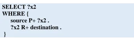
SELECT ?x2 WHERE {
source P+ ?x2 . ?x2 R+ destination . }
Figure 6. The above SPARQL query lists all the nodes x2 for which there exists a P-path from source to x2 and an R-path from x2 to destination. Again, both paths are of length at least one.
The query Q lists the ordered triples (x1, x2, x3) such that there exists a P-path from x1 to x2 and an R-path from x2 to x3. More formally, applying Q to the dataset D produces the answer set Q(x1, x2, x3)[D] = {(x1, x2, x3) : x1⇒Px2 and x2⇒R x3}. By simultaneously substituting the constants source and destination for all occurrences of the projection variables x1 and x3 in Q, we get the resulting query Q´(x2) = Q(x1, x2, x3){ x1|source, x3|destination} shown in Figure 6. It is easy to see that the answer set of Q´ is precisely {x2 : source⇒Px2 and x2⇒Rdestination}.
What this means in terms of efficiency, is that instead of evaluating two queries, each involving two projection variables, and then computing their join, we can, equivalently, evaluate a single query, involving one projection variable. This approach has the potential to reduce
the computational cost significantly. ▲
It is important to point out that this technique is not only valid for just two relevant queries but it can be readily generalized to an arbitrary (finite) number of relevant queries, due to the transitive nature of the ~ relation.
5.CONCLUSION
In this paper we have analyzed SPARQL queries using concepts and ideas inspired from the field of abstract mathematics. This novel approach, besides its theoretical merits, has the potential to provide important practical benefits regarding the computational aspects of SPARQL query evaluation. Quite often in practice we may encounter composite queries that are comprised of simpler queries that happen to be relevant. This situation was demonstrated in the toy scale Example 4, where the evaluation of the conjunction of two SPARQL queries was considered. The current approach requires the evaluation of both queries in order to achieve the evaluation of their conjunction. Knowledge of the fact that the queries in question happen to be relevant, along with a covering query establishing their relation, opens up another possibility. By using only one query, specifically one arising from the covering query via an appropriate substitution, the evaluation of the conjunction can be completed in a more efficient manner, requiring less computational time.
REFERENCES
[image:7.595.326.550.72.136.2][2] Resource Description Framework (RDF), http://www.w3.org/standards/techs/rdf#w3c_all.
[3] SPARQL 1.1 Query Language. Tech. rep., W3C (2013), http://www.w3.org/TR/#tr_SPARQL/.
[4] Wang Y., Liu J., Chen J., Huang Y.: Finding similar queries based on query representation analysis. World Wide Web, vol. 17, n. 5, pp. 1161–1188, Sep. 2014.
[5] Yanan Li, Bin Wang, Sheng Xu, Peng Li, Jintao Li: QueryTrans: Finding Similar Queries Based on Query Trace Graph. In: Proceedings of the 2009 IEEE/WIC/ACM International Joint Conference on Web Intelligence and Intelligent Agent Technology, Vol. 01, Washington, DC, USA, 2009.
[6] Schmidt M., Meier M., Lausen G.: Foundations of SPARQL Query Optimization. In: Proceedings of the 13th International Conference on Database Theory (ICDT '10), pp. 4–33, Lausanne, Switzerland, 2010.
[7] Zhang, X., Feng, Z., Wang, X., Rao, G., Wu, W.: Context-free path queries on RDF graphs. In: International Semantic Web Conference. pp. 632–648. Springer (2016).
[8] Sistla, A.P., Hu, T., Chowdhry, V.: Similarity based retrieval from sequence databases using automata as queries. In:
Proceedings of the eleventh international conference on Information and knowledge management. pp. 237–244. ACM (2002).
[9] Wang, X., Ling, J., Wang, J., Wang, K., Feng, Z.: Answering provenance-aware regular path queries on RDF graphs using an automata-based algorithm. In: Proceedings of the 23rd International Conference on World Wide Web. pp. 395–396. ACM (2014).
[10] Giannakis, K., Andronikos, T.: Querying Linked Data and B¨uchi automata. In: Semantic and Social Media Adaptation and Personalization (SMAP), 2014 9th International Workshop on. pp. 110–114. IEEE (2014).
[11] Giannakis, K., Theocharopoulou, G., Papalitsas, C., Andronikos, T., Vlamos, P.: Associating -automata to path queries on webs of linked data. Engineering Applications of Artificial Intelligence 51, 115 – 123 (2016).