Coverage and Connectivity Probabilities in WSN with Heterogeneous Capability Nodes

! "

# # "$ % %#

& ''' (

Coverage and Connectivity Probabilities in WSN with Heterogeneous Capability Nodes

G.N. Purohit

Centre for Mathematical Sciences Banasthali University Banasthali-304022, INDIA gn_purohitjaipur @yahoo.co.in

Seema Verma

Department of Electronics, AIM & ACT Banasthali University

Banasthali-304022, INDIA [email protected]

Megha Sharma*

Department of Computer Science, AIM & ACT Banasthali University

Banasthali-304022, INDIA [email protected]

Abstract: A sensor network provides flexible communication network, which can be deployed rapidly over wide and/or inaccessible areas. However, the need to gather data from all sensors in the network imposes constraints on the distances between sensors.In a WSN, after collecting information from the environment, sensors need to transmit aggregated data to gateways or information collection nodes. It is important to ensure that every sensor can communicate with the gateways. This leads to the need for sufficient connectivity in addition to optimal coverage. In this paper we consider a heterogeneous sensor network that addresses the problem of coverage and connectivity together, however, in the earlier studies the case of homogeneous sensors was considered. A combination of sensors of higher capabilities (communicating, sensing) and lower capabilities gives better results compared to deployment of only homogeneous sensors. It is ensured that both the coverage and connectivity of the system are maintained. In particular, we are interested in maintaining connected WSNs that effectively cover the Region of Interest (R.O.I). Our sensors can be in alert or sleeping mode. We compute the probabilities for the sensor to stay in the off, sense/receive, and transmit state ensuring coverage and connectivity in the network. We develop the Markov model and its solution for steady state.

Keywords: sensing nodes; heterogeneous; coverage; connectivity; probability

I. INTRODUCTION

Recent advancements in microelectronics, digital signal processing, and low-power RF techniques have enabled the deployment of large wireless sensor networks. Wireless sensor networks can be deployed in areas without infrastructure support, in hostile fields, and under harsh environments. A wireless sensor network consists of many nodes generally communicating through radio waves. The sensors are not integrated into any existing network architecture, so they communicate through a network of ad hoc wireless connections. In the past, sensors were connected by wired lines. Today, this environment is combined with the novel ad hoc networking technology to facilitate inter-sensor communication [1, 4]. The flexibility of installing and configuring a sensor network is thus greatly improved.

Coverage and connectivity are the fundamental requirements in wireless sensor networks and can be considered the metrics of interest when targeting quality of service for applications which are considered in many operations of sensor networks, including, clustering, synchronization, query and information discovery, deployment and redeployment. Coverage is the area or the number of targets that can be monitored by a sensor. On the other hand, connectivity ensures that sensor nodes can communicate with each other in order to aggregate data reports to the base stations (sinks). The wireless communication in WSNs can be either ad hoc (multi-hop) or

single-hop wireless transmission [3]. We consider a wireless ad hoc network (or sensor network), where each wireless node has a maximum transmission power so that it can send signals to all nodes within its transmission range.

In this paper we focus on the coverage and connectivity issues of heterogeneous two-dimensional networks, where the nodes have different sensing and transmission range. The general probabilistic Markov model is presented, in which each sensor node makes an independent decision regarding which state to be in at a given instance. This model is illustrated using a three state model with a transmit (T), receive/sense (S) and off state (O), and the nodes can be in any of the three states at any given point of time. Node makes transitions between the states which are governed by a set of parameters.

The remaining paper is organized as follows. Section II gives the Markov Model for the state probabilities of a sensor node. In Section III the Sensor Coverage and connectivity are studied. In section IV the Numerical Results are presented graphically. Section V concludes the paper.

II. THE MARKOV MODEL

If

2 1

and

S

S

r

r

are the sensing radii of type I and type II nodes respectively and

2 1

and

r

T

r

_T are the transmission

radii of type I and type II nodes respectively, then the combined sensing and transmission radii for both the type I and type II nodes are computed as weighted average of

1

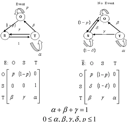
The three states that a node can remain in are the off (O), the sense/receive (S), and the transmit (T) states. The transition of a node from one state to another depends on its environment, which can be in either of the two states: (i) a sense/ receive event is occurring or (ii) no such event is occurring. The Markov state diagram and the transition

probability matrices, E when there is an event and

E

when there is no event are given below.

Figure 1. Markov state diagram and transition probability matrices

In case of a sensing event, the nodes makes a transition to the transmit state. In case of both sensing and receiving events node always attempts to transmit the sensed event rather than the received event. We denote

pr

_O

,

pr

_S

pr

_T as the respective probabilities of the nodes in off, sense/receiving and transmit states. These three probabilities

can be collectively denoted as a vector At any point of time an event can be either sensing or

receiving. The probabilities of an event will therefore depend on the probability that a single neighbor is

transmitting. If we suppose now, that the, system has equilibrated to steady state, in which

(

1

)

pr

( )

pr

S

pr

t

+

=

t

=

,

where

p

S the probability in the steady state We also make the mean field approximation that all the neighbors of the node are in the same steady state and can transmission radius is

P

_REV, then assuming that the sensing disks are in unit torus, the probability that a node is within finally arrive at the following equation for

P

_REV:

(

)

₂

(

₂

)

N 2

Since, the sensing and receiving events are independent

[

Sense

or

receive

]

expression to solve equation (1)

For the steady state probabilities

P

s , we

T

Theorem 1. The set of non- linear steady state equations for

S type I and type II nodes respectively

.

A. Coverage given node is sensing and within the sensing radius of

y

is

S

Under the independent assumption that no node can sense an even at y is then, given by

Which is the probability that y is not covered either by type I nodes or by type II nodes.

We define the coverage function by,

( )

=

Let A be the area that is not covered, then to the following proposition.

Proposition 2 Let 2

( )

n

₁

/

n

₁

Then the expected coverage is given by

( )

power used by the sensing nodes.

where

µ

( )

N

=

N

π

r

_S2

pr

_S,

Proof: We give proof in the appendix

.

B. Connectivity

If a sensing event occurs at some position

y

∈

R

, and we wish to transmit the occurrence of this event to

z

∈

R

, then we would like to successfully transmit the occurrence of this event for any y, z. i.e., we would want the probability for successful transmission to be high.

A path exists from y to z if there is a sequence of nodes in the receiving state at locations l0, l1, ... , lM such that

T1:

y

−

l

₀

≤

r

_s y can be sensed T2:

l

_i

−

l

_i−1

≤

r

_T

For i=1,...,M

Therefore the event can be transmitted from

l

_i−1 to

l

_i, and

it will be received since

l

_i is in the receiving state.

T3:

l

_M

−

z

≤

r

_T (

l

_M can transmit to z)

When,

l

₀ transmits to

l

₁, it is necessary that

l

₁ is in

the sensing state and no their node that is within transmission range of

l

₁ is also attempting to transmit, and

similarly for every path/link

l

_i−1,

l

_i in the path. If there exists such a contention free path for any y, z then we can say that the sensor network is transmission connected. Connectivity here implies coverage as well i.e., the network covers the area as well. For y to be covered, the same nodes need to cover the area with respect to

r

_s . But to guarantee that y is reachable or can be transmitted to it is necessary that the sensing nodes cover the area with respect to

r

_T as well. Thus, we apply the results of the previous section on coverage with

r

_S,

r

_T replaced by

r

=

min

{

r

_S

,

r

_T

}

. This leads to the following result.

Proposition 4. Let A’ be the area that cannot be transmitted to and let A be the area not covered. Then, for any

∈>

0

.

( )

( ) ( )

( )

N

,

'

1

2

'

A

A

Pr

N ' 5 N

' 10 1

−

≥

≤

∪

∈ − ∈

− −

µ

µ π µ

π

O

e

e

where

µ

'

( )

N

=

N

π

r

2

pr

_S,

Proof: The claim follows from Theorem 3 and the observation that if

r

_s

≤

r

_T or , then

A

∪

A'

⊆

A

, otherwise

A

∪

A'

⊆

A'

.

Therefore the coverage results should imply conditions T1 and T3 of path connectivity. Now, we consider requirement T2. For this requirement, it is sufficient that the sensing disk graph obtained by taking disks with radii

r

_T centered at the sensing nodes be connected. Such results were developed in [5] for the case where N nodes are uniformly scattered on an area D, each having radius

r

( )

N

. A small complication here is that while N nodes are scattered, only about

N

pr

_S

of them are sensing. In [13] the following result is proved.

Theorem 5.([5]) The probability that the random sensing disk graph is connected asymptotically approaches 1 if and

only if

π

r

2

( )

N

=

(

log

N

+

c

( )

N

)

/

N

where

c

( )

N

→

∞

It is also known that in grid-disk graphs, with unreliable nodes, the results are very similar to the random node placement [9], and in this case it is known that the number

of hops required is of order

N

/

log

N

.We expect that such results should hold in our case as well.

Theorem 6. Let

r

( )

N

=

min

{

r

_s

( ) ( )

N

,

r

_T

N

}

And for any

0

<∈<

1

, let

N

( ) (

∈

=

1

−

∈

)

N

p

_S,. Let P be the area that is path connected. If

(i) 2

( )

N

N

→

∞

,

S

pr

r

π

and

(ii)

π

r

2

( ) ( )

N

N

∈

=

log

(

N

( )

∈

+

c

(

N

( )

∈

)

)

,

( )

∞

→

∞

=

m

,

m

pr

lim

Then, for any

[

]

∞

→

=

−

≥

>

N

.

1

1

C

Pr

lim

,

0

η

η

,

Proof. The proof is provided as an appendix of this paper.

In order to address the contention problem we present a heuristic which we refer to as

ρ

−

flooding

. We require that in the event that a node needs to transmit the message, the expected number of recipients will be given by

ρ

>

1

. In such a case we can see that the particular message will rapidly flood through the network and we can expect the message to spread exponentially fast. Since there are

N

_S nodes, we can expect that in order of

ρ

log

/

N

S

N

log

/

N

. The requirement of

ρ

−

flooding

sets constraints on the allowable parameters in the Markov model, which is what we derive here.

Let’s consider the situation when a node is in the transmission state, and let be any one of the other N-1 nodes. Let

Q

be the probability to successfully transmit the

packet to , then

Pr

_SUCCESS

=

π

r

_T2

Q

. To achieve successful transmission given that is within transmission range, either the first trial was successful, or the first trial was not successful, and some trial after the first trial was successful. Since the process is Markov and since the nodes are independent, the probability that some trial after the first one is successful is also Q. Let Q1 be the probability

that we are successful on the first trial given that is within transmission range. Since the probability to remain transmitting is

α

, we have

Q

=

Q

₁

+

(

1

−

Q

₁

)

α

Q

or

1 1

1

Q

Q

Q

α

α

+

−

=

(7)

Suppose that has M neighbors. then we are successful on the first trial if is in the sensing state and no other neighbor of is transmitting, which occurs with probability

(

1

_T

)

M

.

S

pr

pr

−

Multiplying

pr

_S

(

1

−

pr

_T

)

M by Pr(M),

summing over M using the fact that M has Binomial

distribution

BD

(

M

;

N

−

2

,

π

r

_T2

)

, we arrive at

(

₂

)

N 2

1

1

−

−

=

pr

_S

r

_T

pr

_T

Q

π

. Since, there are

N-1 nodes to which we could transmit, the expected number of successful transmissions is given by (N-1)

pr

_SUCCESS. Requiring that the expected number of successful transmissions is then leads to the following constraint.

Proposition 7. In order to achieve

ρ

−

flooding

, the following condition must be satisfied,

(

)

(

)

( )

(

₂

)

(N 2)

2 N 2 2

-1

1

-1

1

N

1 1

− −

+

−

−

=

T T S

T T S

T

pr

r

pr

pr

r

r

p

r

π

α

α

π

π

ρ

IV. NUMERICAL RESULTS

Figure 2 compares the steady state probabilities calculated for different network sizes comprising of different ratios of type I and type II nodes. For the ratio 1:4 of type I and type II nodes the transmission/sensing radius are kept constant at 0.05 _and 0.35 _{for type I and type II}

nodes respectively, and the sensing event probabilities

SEV

P

are kept constant at 0.4 _and 0.65 _{for type I and type}

II nodes respectively.

For the ratio 1:3 of type I and type II nodes the transmission/sensing radius are kept constant at 0.1 and 0.3 for type I and type II nodes respectively, and the sensing

event probabilities

P

_SEV are kept constant at 0.4 and 0.6 for type I and type II nodes respectively.

For the ratio 1:2 of type I and type II nodes the transmission/sensing radius are kept constant at 0.16 _and 0.25 _{for type I and type II nodes respectively, and the}

sensing event probabilities

P

_SEV are kept constant at 0.4

and 0.55 _{for type I and type II nodes respectively.}

We can observe that the number of nodes in the off state increases as the network increases and the number of nodes in the sense/receive state decreases with an increase in the network size.

Fig.ure 2.The steady state probabilities for different network sizes and different ratios type I and type II sensor nodes. The probabilities for off state and sense/receive state are shown, whereas the probability for the

transmission state is

pr

_T

=

1

−

pr

_O

−

pr

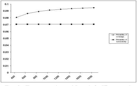
_S

Figure 3 presents the coverage and connectivity results. We can observe that the overall coverage and connectivity is well maintained with the increasing number of nodes. Although the number of nodes in the sense/receive state decreases with the increase in network size, as can be seen in Fig. 2 but the number of sensing nodes if high enough to maintain the coverage and connectivity with a high probability, i.e., the number of sensing nodes is optimal as required.

Figure 3. The coverage and connectivity graphs for different network sizes for the ration 1:3 of type I and type II nodes.

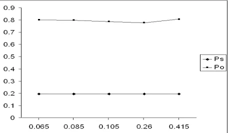
Figure 4.The Steady state probabilities for different values of sensing event probability, for a network of size 600, for the ratio 1:3 of type I and type II

nodes

V. CONCLUSION

The probabilities for staying in the off, sense/receive, transmit state for a heterogeneous (the nodes have different sensing range and transmission range) two dimensional network are calculated and represented graphically which ensure both coverage and connectivity. A general probabilistic Markov model is proposed in which each sensor node makes an independent decision regarding which state to be in at a given time and is illustrated using a three state model with a transmit, receive/sense and off state, and the nodes can be in either of the three states at any given point of time viz. transmit, receive/sense and off state.

VI.REFERENCES

[1] G. J. Pottie and W. J. Kaiser, “Wireless integrated network sensors.” Commun. ACM, Vol. 43, No. 5, pp. 51–58, 2000.

[2] J.Franklin, “Mathematical Methods of Economics,” Springer Verlag, New York, 1980.

[3] K. Sohraby, D. Minoli, and T. Znati, “Wireless Sensor Networks: Technology, Protocols and Applications” John Wiley & Sons, Inc.: Hoboken, NJ, USA, 2007.

[4] K. Sohrabi, J. Gao, V. Ailawadhi, and G. J. Pottie, “Protocols for self-organization of a wireless sensor network,” IEEE Personal Commun., Vol. 7, No. 5, pp.16–27, 2000.

[5] P. Gupta and P.R. Kumar, “Critical power for asymptotic connectivity in wireless networks,” in: Stochastic Analysis, Control, Optimization and Applications, A Volume in Honor of W.H. Fleming. Edited by W.M. Mc Eneany, G. Yin, and Q. Zhang (Birkhauser), pp. 547-566, 1998.

[6] R. Motwani and P. Raghavan, “Randomized Algorithms,”

[7] Cambridge University Press, Cambridge, UK, 2000.

[8] S. Shakkattai, R. srikant, and N. Shroff, “Unrealiabale sensor grids:Coverage, connectivity and diameter,” in Proceedings of IEEE INFOCOM’03, 2003

VII. APPENDIX

Proof of Theorem 3. We can inscribe a square of

side

∆

=

r

_S

2

in

a

circle

of

radius

r

_S . The coverage by disks will then be no less then the coverage by the squares. Let A’ be the area not covered by the squares, then G U. Defining the coverage function

f

_A

( )

y

for the squares analogously to (4), we find that

[ ]

A

(

1

2

pr

_S

)

N

E

=

−

∆

.

E

[ ]

A

2

=

dy

dz

f

_A

( ) ( )

y

f

_A

z

.The

f

_a

( ) ( )

y

f

_A

z

term in the integrand is the probability that both points y and z are not covered. Let

A

_W denote the square centered at the

point

W

∈

R

.

Then the probability that both points y and z

(in the integrand) are not covered is given by the probability that all the sensing squares are outside

A

_x

A

_y , so

[ ]

₂

(

)

N

A

A

1

A

1

−

=

dy

dz

p

_{S x y}

E

. In the integral,

let

y

=

(

y

₁

,

y

₂

)

and

z

=

(

z

₁

,

z

₂

)

If

y

₁

−

z

₁

≥

∆

or

∆

≥

−

₂

2

z

y

then

A

_y

A

_z

=

2

∆

2

.

Otherwise,

(

1 1

)(

2 2

)

2

.

2

A

A

_{y z}

=

∆

−

∆

−

y

−

z

∆

−

y

−

z

. Fix

z in the y integral. The area over which z can range with

z

A

disjoint from

A

_y is

1

−

4

∆

2 . This area thus

contributes

(

1

−

4

∆

2

)(

1

−

2

∆

2

)

N to the integral. Over the

remaining area, changing coordinate in the

z

integral so that its origin lies at y, this contribution to the integral (over the area when two squares overlap) becomes

(

)(

)

(

)

∆

≤

≤

−

∆

−

∆

+

∆

−

=

2 1

N

2 1

2

,

z

0

2

1

4

z

z

z

pr

pr

dz

dy

I

_{S S}

,

A computation to perform these integrals then leads to the following result, after adding the contribution from the part of the integral over the region where

A

_y and

A

_z are

disjoint.

[ ]

(

)

(

1

)

,

N

4

1

2

1

A

2 i N

1 2 N

2 2

+

∆

+

∆

−

=

=

i

i

pr

pr

E

i S S

where

λ

=

pr

_S

∆

2

/

(

1

−

2

pr

_S

∆

2

)

. Using the fact that

( )

[ ]

2

[ ]

2

A

A

A

var

=

E

−

E

and

[ ]

A

2

=

(

1

−

2

pr

_S

∆

2

) (

N

1

+

pr

_S

∆

2

λ

)

N

,

( )

(

)

We can now apply the Markov inequality to Ato get

connected on a sufficiently large area, with probability 1 in the asymptotic limit.

AUTHORS

Prof. G. N. Purohit is a Professor in Department of Mathematics & Statistics at Banasthali University (Rajasthan). Before joining Banasthali University, he was Professor and Head of the Department of Mathematics, University of Rajasthan, Jaipur. He had been Chief-editor of a journal.His present interest is in O.R., Discrete Mathematics and Communication networks. He has published around 40 research papers in various journals.

Mrs. (Dr.) Seema Verma obtained her M.Tech and Ph.D degree from Banasthali University in 2003 and 2006 respectively. She is a associate Professor of Electronics. Her research areas are VLSI Design, communication Networks. She has published around 18 research papers in various Journals.