Parallel Implementations of Word Alignment Tool
Qin Gao and Stephan Vogel Language Technology Institution
School of Computer Science Carnegie Mellon University Pittsburgh, PA, 15213, USA
{qing, stephan.vogel}@cs.cmu.edu
Abstract
Training word alignment models on large cor-pora is a very time-consuming processes. This paper describes two parallel implementations of GIZA++ that accelerate this word align-ment process. One of the implementations runs on computer clusters, the other runs on multi-processor system using multi-threading technology. Results show a near-linear speed-up according to the number of CPUs used, and alignment quality is preserved.
1 Introduction
Training state-of-the-art phrase-based statistical ma-chine translation (SMT) systems requires several steps. First, word alignment models are trained on the bilingual parallel training corpora. The most widely used tool to perform this training step is the well-known GIZA++(Och and Ney, 2003). The re-sulting word alignment is then used to extract phrase pairs and perhaps other information to be used in translation systems, such as block reordering mod-els. Among the procedures, more than 2/3 of the time is consumed by word alignment (Koehn et al., 2007). Speeding up the word alignment step can dramatically reduces the overall training time, and in turn accelerates the development of SMT systems.
With the rapid development of computing hard-ware, multi-processor servers and clusters become widely available. With parallel computing, process-ing time (wall time) can often be cut down by one or two orders of magnitude. Tasks, which require several weeks on a single CPU machine may take only a few hours on a cluster. However, GIZA++
was designed to be single-process and single-thread. To make more efficient use of available computing resources and thereby speed up the training of our SMT system, we decided to modify GIZA++ so that it can run in parallel on multiple CPUs.
The word alignment models implemented in GIZA++, the so-called IBM (Brown et al., 1993) and HMM alignment models (Vogel et al., 1996) are typ-ical implementation of the EM algorithm (Dempster et al., 1977). That is to say that each of these mod-els run for a number of iterations. In each iteration it first calculates the best word alignment for each sentence pairs in the corpus, accumulating various counts, and then normalizes the counts to generate the model parameters for the next iteration. The word alignment stage is the most time-consuming part, especially when the size of training corpus is large. During the aligning stage, all sentences can be aligned independently of each other, as model parameters are only updated after all sentence pairs have been aligned. Making use of this property, the alignment procedure can be parallelized. The basic idea is to have multiple processes or threads aligning portions of corpus independently and then merge the counts and perform normalization.
The paper implements two parallelization meth-ods. The PGIZA++ implementation, which is based on (Lin et al, 2006), uses multiple aligning cesses. When all the processes finish, a master pro-cess starts to collect the counts and normalizes them to produce updated models. Child processes are then restarted for the new iteration. The PGIZA++ does not limit the number of CPUs being used, whereas it needs to transfer (in some cases) large amounts
of data between processes. Therefore its perfor-mance also depends on the speed of the network in-frastructure. The MGIZA++ implementation, on the other hand, starts multiple threads on a common ad-dress space, and uses a mutual locking mechanism to synchronize the access to the memory. Although MGIZA++ can only utilize a single multi-processor computer, which limits the number of CPUs it can use, it avoids the overhead of slow network I/O. That makes it an equally efficient solution for many tasks. The two versions of alignment tools are available on-line at http://www.cs.cmu.edu/˜qing/giza.
The paper will be organized as follows, section 2 provides the basic algorithm of GIZA++, and sec-tion 3 describes the PGIZA++ implementasec-tion. Sec-tion 4 presents the MGIZA++ implementaSec-tion, fol-lowed by the profile and evaluation results of both systems in section 5. Finally, conclusion and future work are presented in section 6.
2 Outline of GIZA++
2.1 Statistical Word Alignment Models
GIZA++ aligns words based on statistical models. Given a source stringfJ
1 =f1,· · ·, fj,· · ·, fJand a
target stringeI1 =e1,· · ·, ei,· · ·, eI, an alignmentA
of the two strings is defined as(Och and Ney, 2003):
A ⊆ {(j, i) :j= 1,· · ·, J;i= 0,· · ·, I} (1)
in case thati = 0in some (j, i) ∈ A, it represents that the source word j aligns to an “empty” target worde0.
In statistical world alignment, the probability of a source sentence given target sentence is written as:
P(f1J|e
1 denotes the alignment on the
sen-tence pair. In order to express the probability in statistical way, several different parametric forms of
P(fJ
1, aJ1|eI1) =pθ(f1J, aJ1|eI1)have been proposed,
and the parametersθ can be estimated using maxi-mum likelihood estimation(MLE) on a training cor-pus(Och and Ney, 2003).
ˆ
The best alignment of the sentence pair,
ˆ
aJ1 = arg max
aJ
1
pθˆ(f1J, aJ1|eI1) (4)
is called Viterbi alignment.
2.2 Implementation of GIZA++
GIZA++ is an implementation of ML estimators for several statistical alignment models, including IBM Model 1 through 5 (Brown et al., 1993), HMM (Vo-gel et al., 1996) and Model 6 (Och and Ney, 2003).
Although IBM Model 5 and Model 6 are sophisti-cated, they do not give much improvement to align-ment quality. IBM Model 2 has been shown to be inferior to the HMM alignment model in the sense of providing a good starting point for more complex models. (Och and Ney, 2003) So in this paper we focus on Model 1, HMM, Model 3 and 4.
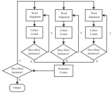
When estimating the parameters, the EM (Demp-ster et al., 1977) algorithm is employed. In the E-step the counts for all the parameters are col-lected, and the counts are normalized in M-step. Figure 1 shows a high-level view of the procedure in GIZA++. Theoretically the E-step requires sum-ming over all the alignments of one sentence pair, which could be(I+ 1)J alignments in total. While (Och and Ney, 2003) presents algorithm to imple-ment counting over all the alignimple-ments for Model 1,2 and HMM, it is prohibitive to do that for Models 3 through 6. Therefore, the counts are only collected for a subset of alignments. For example, (Brown et al., 1993) suggested two different methods: us-ing only the alignment with the maximum probabil-ity, the so-called Viterbi alignment, or generating a set of alignments by starting from the Viterbi ment and making changes, which keep the align-ment probability high. The later is called “pegging”. (Al-Onaizan et al., 1999) proposed to use the neigh-bor alignments of the Viterbi alignment, and it yields good results with a minor speed overhead.
During training we starts from simple models use the simple models to bootstrap the more complex ones. Usually people use the following sequence: Model 1, HMM, Model 3 and finally Model 4. Table 1 lists all the parameter tables needed in each stage and their data structures1. Among these models, the
1
In filename, prefix is a user specified parameter, andnis
Figure 1: High-level algorithm of GIZA++
lexicon probability table (TTable) is the largest. It should contain all thep(fi, ej)entries, which means the table will have an entry for every distinct source and target word pairfi, ej that co-occurs in at least one sentence pair in the corpus. However, to keep the size of this table manageable, low probability en-tries are pruned. Still, when training the alignment models on large corpora this statistical lexicon often consumes several giga bytes of memory.
The computation time of aligning a sentence pair obviously depends on the sentence length. E.g. for IBM 1 that alignment is O(J ∗I), for the HMM alignment it is O(J +I2
), with J the number of words in the source sentence andI the number of words in the target sentence. However, given that the maximum sentence length is fixed, the time com-plexity of the E-step grows linearly with the num-ber of sentence pairs. The time needed to perform the M-step is dominated by re-normalizing the lexi-con probabilities. The worst case time complexity is
O(|VF| ∗ |VE|), where|VF|is the size of the source vocabulary and|VE|is the size of the target vocabu-lary. Therefore, the time complexity of the M-step is polynomial in the vocabulary size, which typically grows logarithmic in corpus size. As a result, the alignment stage consumes most of the overall pro-cessing time when the number of sentences is large. Because the parameters are only updated during the M-step, it will be no difference in the result whether we perform the word alignment in the E-step sequentially or in parallel2. These
character-2
However, the rounding problem will make a small
differ-istics make it possible to build parallel versions of GIZA++. Figure 2 shows the basic idea of parallel GIZA++.
Figure 2: Basic idea of Parallel GIZA++
While working on the required modification to GIZA++ to run the alignment step in parallel we identified a bug, which needed to be fixed. When training the HMM model, the matrix for the HMM trellis will not be initialized if the target sentence has only one word. Therefore some random numbers are added to the counts. This bug will also crash the system when linking against pthread library. We observe different alignment and slightly lower per-plexity after fixing the bug3.
3 Multi-process version - PGIZA++
3.1 Overview
A natural idea of parallelizing GIZA++ is to sep-arate the alignment and normalization procedures, and spawn multiple alignment processes. Each pro-cess aligns a chunk of the pre-partitioned corpus and outputs partial counts. A master process takes these counts and combines them, and produces the nor-malized model parameters for the next iteration. The architecture of PGIZA++ is shown in Figure 3.
ence in the results even when processing the sentences sequen-tially, but in different order.
3
Model Parameter tables Filename Description Data structure Model 1 TTable prefix.t1.n Lexicon Probability Array of Array
HMM TTable prefix.thmm.n
ATable prefix.ahmm.n Align Table 4-D Array
HMMTable prefix.hhmm.n HMM Jump Map
Model 3/4 TTable prefix.t3.n
ATable prefix.a3.n Align Table
NTable prefix.n3.n Fertility Table 2-D Array
DTable prefix.d3.n Distortion Table 4-D Array
pz prefix.p0 3.n Probability for null wordsp0 Scalar (Model 4 only) D4Table prefix.d4.nprefix.D4.n Distortion Table for Model 4 Map
Table 1: Model tables created during training
Figure 3: Architecture of PGIZA++
3.2 Implementation
3.2.1 I/O of the Parameter Tables
In order to ensure that the next iteration has the correct model, all the information that may affect the alignment needs to be stored and shared. It includes model files and statistics over the training corpus. Table 1 is a summary of tables used in each model.
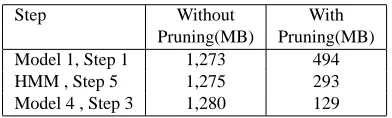
Step Without With
Pruning(MB) Pruning(MB) Model 1, Step 1 1,273 494 HMM , Step 5 1,275 293 Model 4 , Step 3 1,280 129
Table 2: Comparison of the size of count tables for the lexicon probabilities
In addition to these models, the summation of “sentence weight” of the whole corpus should be stored. GIZA++ allows assigning a weight wi for each sentence pairsisto indicate the number of oc-currence of the sentence pair. The weight is
normal-ized bypi = wi/Piwi, so that Pipi = 1. Then thepi serves as a prior probability in the objective function. As each child processes only see a portion of training data, it is required to calculate and share theP
iwi among the children so the values can be consistent.
The tables and count tables of the lexicon proba-bilities (TTable) can be extremely large if not pruned before being written out. Pruning the count tables when writing them into a file will make the result slightly different. However, as we will see in Sec-tion 5, the difference does not hurt translaSec-tion per-formance significantly. Table 2 shows the size of count tables written by each child process in an ex-periment with 10 million sentence pairs, remember there are more than 10 children writing the the count tables, and the master would have to read all these tables, the amount of I/O is significantly reduced by pruning the count tables.
3.2.2 Master Control Script
The other issue is the master control script. The script should be able to start processes in other nodes. Therefore the implementation varies accord-ing to the software environment. We implemented three versions of scripts based on secure shell, Con-dor (Thain et al., 2005) and Maui.
3.3 Advantages and Disadvantages
One of the advantages of PGIZA++ is its scalability, it is not limited by the number of CPUs of a sin-gle machine. By adding more nodes, the alignment speed can be arbitrarily fast4. Also, by splitting the corpora into multiple segments, each child process only needs part of the lexicon, which saves mem-ory. The other advantage is that it can adopt differ-ent resource managemdiffer-ent systems, such as Condor and Maui/Torque. By splitting the corpus into very small segments, and submitting them to a scheduler, we can get most out of clusters.
However, PGIZA++ also has significant draw-backs. First of all, each process needs to load the models of the previous iteration, and store the counts of the current step on shared storage. Therefore, I/O becomes a bottleneck, especially when the num-ber of child processes is large. Also, the normal-ization procedure needs to read all the count files from network storage. As the number of child pro-cesses increases, the time spent on reading/writing will also increase. Given the fact that the I/O de-mand will not increase as fast as the size of corpus grows, PGIZA++ can only provide significant speed up when the size of each training corpus chunk is large enough so that the alignment time is signifi-cantly longer than normalization time.
Also, one obvious drawback of PGIZA++ is its complexity in setting up the environment. One has to write scripts specially for the scheduler/resource management software.
Balancing the load of each child process is an-other issue. If any one of the corpus chunks takes longer to complete, the master has to wait for it. In other words, the speed of PGIZA++ is actually de-termined by the slowest child process.
4 Multi-thread version - MGIZA++
4.1 Overview
Another implementation of parallelism is to run sev-eral alignment threads in a single process. The threads share the same address space, which means it can access the model parameters concurrently without any I/O overhead.
4
The normalization process will be slower when the number of nodes increases
The architecture of MGIZA++ is shown in Figure 4.
Data Sentence
Provider
Thread 1 Thread 2 Thread n
Synchronized Assignment of Sentence Pairs
Model
Synchronized Count Storage
Main Thread
Normalization
Figure 4: Architecture of MGIZA++
4.2 Implementation
The main thread spawns a number of threads, us-ing the same entry function. Each thread will ask a provider for the next sentence pair. The sentence provider is synchronized. The request of sentences are queued, and each sentence pair is guaranteed to be assigned to only one thread.
Table Synchronizations Method TTable Write lock on every target words ATable Duplicate/Merge
HMMTable Duplicate/Merge DTable Duplicate/Merge NTable Duplicate/Merge D4Table Duplicate /Merge Perplexity Mutual lock
Table 3: Synchronizations for tables in MGIZA++
Each thread outputs the alignment into its own output file. Sentences in these files are not in sequen-tial order. Therefore, we cannot simply concatenate them but rather have to merge them according to the sentence id.
4.3 Advantages and Disadvantages
Because all the threads within a process share the same address space, no data needs to be transferred, which saves the I/O time significantly. MGIZA++ is more resource-thrifty comparing to PGIZA++, it do not need to load copies of models into memory.
In contrast to PGIZA++, MGIZA++ has a much simpler interface and can be treated as a drop-in replacement for GIZA++, except that one needs to run a script to merge the final alignment files. This property makes it very simple to integrate MGIZA++ into machine translation packages, such as Moses(Koehn et al., 2007).
One major disadvantage of MGIZA++ is also ob-vious: lack of scalability. Accelerating is limited by the number of CPUs the node has. Compared to PGIZA++ on the speed-up factor by each addi-tional CPU, MGIZA++ also shows some deficiency. Due to the need for synchronization, there are al-ways some CPU time wasted in waiting.
5 Experiments
5.1 Experiments on PGIZA++
For PGIZA++ we performed training on an Chinese-English translation task. The dataset consists of ap-proximately 10 million sentence pairs with 231 mil-lion Chinese words and 258 milmil-lion English words. We ran both GIZA++ and PGIZA++ on the same training corpus with the same parameters, then ran Pharaoh phrase extraction on the resulting align-ments. Finally, we tuned our translation systems on the NIST MT03 test set and evaluate them on NIST
MT06 test set. The experiment was performed on a cluster of several Xeon CPUs, the storage of cor-pora and models are on a central NFS server. The PGIZA++ uses Condor as its scheduler, splitting the training data into 30 fragments, and ran training in both direction (Ch-En, En-Ch) concurrently. The scheduler assigns11CPUs on average to the tasks. We ran 5 iterations of Model 1 training, 5 iteration of HMM, 3 Model 3 iterations and 3 Model 4 iter-ations. To compare the performance of system, we recorded the total training time and the BLEU score, which is a standard automatic measurement of the translation quality(Papineni et al., 2002). The train-ing time and BLEU scores are shown in Table 4:5
Running (TUNE) (TEST) Time MT03 MT06 CPUs GIZA++ 169h 32.34 29.43 2 PGIZA++ 39h 32.20 30.14 11
Table 4: Comparison of GIZA++ and PGIZA++
The results show similar BLEU scores when us-ing GIZA++ and PGIZA++, and a 4 times speed up. Also, we calculated the time used in normaliza-tion. The average time of each normalization step is shown in Table 5.
Per-iteration (Avg) Total Model 1 47.0min 235min (3.9h) HMM 31.8min 159min (2.6h) Model 3/4 25.2 min 151min (2.5h)
Table 5: Normalization time in each stage
As we can see, if we rule out the time spent in normalization, the speed up is almost linear. Higher order models require less time in the normalization step mainly due to the fact that the lexicon becomes smaller and smaller with each models (see Table 2. PGIZA++, in small amount of data,
5.2 Experiment on MGIZA++
Because MGIZA++ is more convenient to integrate into other packages, we modified the Moses sys-tem to use MGIZA++. We use the Europal English-Spanish dataset as training data, which contains 900 thousand sentence pairs, 20 million English words and 20 million Spanish words. We trained the
5
English-to-Spanish system, and tuned the system on two datasets, the WSMT 2006 Europal test set (TUNE1) and the WSMT news commentary dev-test set 2007 (TUNE2). Then we used the first pa-rameter set to decode WSMT 2006 Europal test set (TEST1) and used the second on WSMT news com-mentary test set 2007 (TEST2)6. Table 6 shows the comparison of BLEU scores of both systems. listed in Table 6:
TUNE1 TEST1 TUNE2 TEST2 GIZA++ 33.00 32.21 31.84 30.56 MGIZA++ 32.74 32.26 31.35 30.63
Table 6: BLEU Score of GIZA++ and MGIZA++
Note that when decoding using the phrase table resulting from training with MGIZA++, we used the parameter tuned for a phrase table generated from GIZA++ alignment, which may be the cause of lower BLEU score in the tuning set. However, the major difference in the training comes from fix-ing the HMM bug in GIZA++, as mentioned before. To profile the speed of the system according to the number of CPUs it use, we ran MGIZA++ on 1, 2 and 4 CPUs of the same speed. When it runs on 1 CPU, the speed is the same as for the original GIZA++. Table 7 and Figure 5 show the running time of each stage:
4000 5000 6000 7000 8000
m
e
(s
)
Model1 HMM Model3/4
0 1000 2000 3000
1 2 3 4
T
im
CPUS
Figure 5: Speed up of MGIZA++
When using 4 CPUs, the system uses only 41%
time comparing to one thread. Comparing to PGIZA++, MGIZA++ does not have as high an
ac-6
http://www.statmt.org/wmt08/shared-task.html
CPUs M1(s) HMM(s) M3,M4(s) Total(s) 1 2167 5101 7615 14913
2 1352 3049 4418 8854
(62%) (59%) (58%) (59%)
4 928 2240 2947 6140
(43%) (44%) (38%) (41%)
Table 7: Speed of MGIZA++
celeration rate. That is mainly because of the re-quired locking mechanism. However the accelera-tion is also significant, especially for small training corpora, as we will see in next experiment.
5.3 Comparison of MGIZA++ and PGIZA++
In order to compare the acceleration rate of PGIZA++ and MGIZA++, we also ran PGIZA++ in the same dataset as described in the previous section with 4 children. To avoid the delay of starting the children processes, we chose to use ssh to start re-mote tasks directly, instead of using schedulers. The results are listed in Table 8.
M1(s) HMM(s) M3,M4(s) Total(s) MGIZA+1CPU 2167 5101 7615 14913 MGIZA+4CPUs 928 2240 2947 6140 PGIZA+4Nodes 3719 4324 4920 12963
Table 8: Speed of PGIZA++ on Small Corpus
There is nearly no speed-up observed, and in Model 1 training, we observe a loss in the speed. Again, by investigating the time spent in normaliza-tion, the phenomenon can be explained (Table 9):
Even after ruling out the normalization time, the speed up factor is smaller than MGIZA++. That is because of reading models when child processes start and writing models when child processes finish. From the experiment we can conclude that PGIZA++ is more suited to train on large corpora than on small or moderate size corpora. It is also im-portant to determine whether to use PGIZA++ rather than MGIZA++ according to the speed of network storage infrastructure.
5.4 Difference in Alignment
Per-iteration (Avg) Total Model 1 8.4min 41min (0.68h) HMM 7.2min 36min (0.60h) Model 3/4 5.7 min 34min (0.57h)
Total 111min (1.85h)
Table 9: Normalization time in each stage : small data
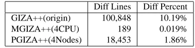
GIZA++ with the bug fixed as the reference. The results of all other systems are listed in Table 10:
Diff Lines Diff Percent GIZA++(origin) 100,848 10.19% MGIZA++(4CPU) 189 0.019% PGIZA++(4Nodes) 18,453 1.86%
Table 10: Difference in Viterbi alignment (GIZA++ with the bug fixed as reference)
From the comparison we can see that PGIZA++ has larger difference in the generated alignment. That is partially because of the pruning on count ta-bles.
To also compare the alignment score in the differ-ent systems. For each sdiffer-entence pairi= 1,2,· · ·, N, assume two systemsbandchave Viterbi alignment scoresSb
The residuals of the three systems are listed in Table 11. The residual result shows that the MGIZA++ has a very small (less than 0.2%) difference in alignment scores, while PGIZA++ has a larger residual.
The results of experiments show the efficiency and also the fidelity of the alignment generated by the two versions of parallel GIZA++. However, there are still small differences in the final align-ment result, especially for PGIZA++. Therefore, one should consider which version to choose when building systems. Generally speaking, MGIZA++ provides smoother integration into other packages: easy to set up and also more precise. PGIZA++ will not perform as good as MGIZA++ on small-size cor-pora. However, PGIZA++ has good performance on large data, and should be considered when building very large scale systems.
6 Conclusion
The paper describes two parallel implementations of the well-known and widely used word alignment
R GIZA++(origin) 0.6503 MGIZA++(4CPU) 0.0017 PGIZA++(4Nodes) 0.0371
Table 11: Residual in Viterbi alignment scores (GIZA++ with the bug fixed as reference)
tool GIZA++. PGIZA++ does alignment on a num-ber of independent processes, uses network file sys-tem to collect counts, and performs normalization by a master process. MGIZA++ uses a multi-threading mechanism to utilize multiple cores and avoid net-work transportation. The experiments show that the two implementation produces similar results with original GIZA++, but lead to a significant speed-up in the training process.
With compatible interface, MGIZA++ is suit-able for a drop-in replacement for GIZA++, while PGIZA++ can utilize huge computation resources, which is suitable for building large scale systems that cannot be built using a single machine.
However, improvements can be made on both versions. First, a combination of the two imple-mentation is reasonable, i.e. running multi-threaded child processes inside PGIZA++’s architecture. This could reduce the I/O significantly when using the same number of CPUs. Secondly, the mechanism of assigning sentence pairs to the child processes can be improved in PGIZA++. A server can take respon-sibility to assign sentence pairs to available child processes dynamically. This would avoid wasting any computation resource by waiting for other pro-cesses to finish. Finally, the huge model files, which are responsible for a high I/O volume can be reduced by using binary formats. A first implementation of a simple binary format for the TTable resulted in files only about 1/3 in size on disk compared to the plain text format.
References
Arthur Dempster, Nan Laird, and Donald Rubin. 1977. Maximum Likelihood From Incomplete Data via the EM Algorithm. Journal of the Royal Statistical Soci-ety, Series B, 39(1):138
Douglas Thain, Todd Tannenbaum, and Miron Livny. 2005. Distributed Computing in Practice: The Con-dor Experience. Concurrency and Computation: Prac-tice and Experience, 17(2-4):323-356
Franz Josef Och and Hermann Ney. 2003. A Systematic Comparison of Various Statistical Alignment Models. Computational Linguistics, 29(1):19-51
Philipp Koehn, Hieu Hoang, Alexandra Birch, Chris Callison-Burch, Marcello Federico, Nicola Bertoldi, Brooke Cowan, Wade Shen, Christine Moran, Richard Zens, Chris Dyer, Ondrej Bojar, Alexandra Con-stantin, Evan Herbst. 2007. Moses: Open Source Toolkit for Statistical Machine Translation. ACL 2007, Demonstration Session, Prague, Czech Repub-lic
Peter F. Brown, Stephan A. Della Pietra, Vincent J. Della Pietra, Robert L. Mercer. 1993. The Mathematics of Statistical Machine Translation: Parameter Estima-tion. Computational Linguistics, 19(2):263-311 Stephan Vogel, Hermann Ney and Christoph Tillmann.
1996. HMM-based Word Alignment in Statistical Translation. In COLING ’96: The 16th International Conference on Computational Linguistics, pp. 836-841, Copenhagen, Denmark.
Xiaojun Lin, Xinhao Wang and Xihong Wu. 2006. NLMP System Description for the 2006 NIST MT Evaluation. NIST 2006 Machine Translation Evalu-ation
Yaser Al-Onaizan, Jan Curin, Michael Jahr, Kevin Knight, John D. Lafferty, I. Dan Melamed, David Purdy, Franz J. Och, Noah A. Smith and David Yarowsky. 1999. Statistical Machine Trans-lation. Final Report JHU Workshop, Available at http://www.clsp.jhu.edu/ws99/projects/mt/final report/mt-final-reports.ps