R E S E A R C H
Open Access
Normalized Bernstein polynomials in
solving space-time fractional diffusion
equation
A Baseri, E Babolian and S Abbasbandy
**Correspondence:
[email protected] Department of Mathematics, Science and Research Branch, Islamic Azad University, Tehran, Iran
Abstract
In this paper, we solve a time-space fractional diffusion equation. Our methods are based on normalized Bernstein polynomials. For the space domain, we use a set of normalized Bernstein polynomials and for the time domain, which is a semi-infinite domain, we offer an algebraic map to make the rational normalized Bernstein functions. This study uses Galerkin and collocation methods. The integrals in the Galerkin method are established with Chebyshev interpolation. We implemented the proposed methods for some examples that are presented to demonstrate the theoretical results. To confirm the accuracy, error analysis is carried out.
Keywords: rational normalized Bernstein functions (RNBF); normalized Bernstein polynomials (NBP); time-space fractional diffusion equation; error analysis; collocation and Galerkin methods
1 Introduction
Fractional calculus allows mathematicians and engineers better modeling of a wide class of systems with anomalous dynamic behavior and better understanding of the facets of both physical phenomena and artificial processes. Hence the mathematical models de-rived from differential equations with noninteger/fractional order derivatives or integrals are becoming a fundamental research issue for scientists and engineers [].
The fractional advection-diffusion equation is presented as a useful approach for the description of transport dynamics in complex systems. The time, space and time-space fractional advection-diffusion equations have been used to describe important physical phenomena that occur in amorphous, colloid, geophysical and geological processes [].
Bernstein polynomials play an important role in many branches of mathematics, such as probability, approximation theory and computer-aided geometric design []. Also, in recent decades, the authors discovered some new analytic properties and some applica-tions for these polynomials. For example, the rate of convergence of these polynomials de-rived by Cheng [] for a certain class of functions. Farouki [] showed that the Bernstein polynomial basis is an optimal stable basis among non-negative bases on the desired in-terval. Alshbool [] approximated solutions of fractional-order differential equations with estimation error by using fractional Bernstein polynomials. Also, he applied a new
ification of the Bernstein polynomial method called multistage Bernstein polynomials to solve fractional order stiff systems [].
In this paper, the normalized Bernstein polynomials with collocation and Galerkin methods are applied to turn the problem into an algebraic system. The fractional diffu-sion equation with variable coefficients is considered
∂βu(x,t)
∂tβ =d(x,t)
∂αu(x,t)
∂xα +b(x,t)
∂γu(x,t)
∂xγ +s(x,t), <x<b,t≥. ()
In this equationu(x,t) is the unknown function,s(x,t) is called the source-term andd(x,t) andb(x,t) are the diffusion and advection coefficients, <α≤ and <γ ≤ are the orders of space fractional derivatives and <β≤ is the time fractional order. We also consider the initial condition
u(x, ) =u(x), <x<b, ()
and the boundary conditions
u(,t) =g(t), u(b,t) =g(t), t≥. ()
The existence and uniqueness of solutions for such problems are guaranteed in [, ]. Note that problem () forα= ,β= andγ = is the classical advection-diffusion equation. Problem () is discussed from the view of some scholars like Gao and Sun [] who propose a numerical algorithm based on the finite difference method forγ = ,α= and Deng [] who discussed in the caseβ= a finite element method with Riemann-Liouville space fractional derivatives.
The structure of this paper is as follows. In Section , some definitions are presented. In Section , normalized Bernstein polynomials and their required properties are given. In Section , we introduce the rational Bernstein functions and also describe some use-ful properties of these basis functions. In Section , the relation between the Legendre polynomials and orthonormal Bernstein is demonstrated. In Section , to estimate the in-tegrals, we introduce a rational Chebyshev interpolation. In Section , Galerkin and collo-cation methods to approximate the unknown functionu(x,t) are applied. In Section , we offer error bounds for integer and fractional derivatives. To show the effectiveness of the proposed method, we report our numerical findings in Section ; and finally, in Section , we give a brief conclusion.
2 Fundamentals of fractional calculus
There are various definitions for fractional derivative and integration. The widely-used definition for a fractional derivative is the Caputo sense and a fractional integration is the Riemann-Liouville definition.
Definition .([]) The Riemann-Liouville fractional integral operator of orderα≥ is defined as follows:
Jαf(x) = (α)
x
(x–t)α–f(t)dt= (α)x
α–∗f(x), α> ,x> , ()
Definition .([]) The Caputo definition of a fractional derivative operator is given by
For simplicity, we denote ∂αi
∂zαibyD
αi
z whichαidenotes the Caputo derivative with respect
toz, note thatαimay beβ,γ orαandzcan bexort.
According to Definition ., the Caputo time and space fractional derivatives of the func-tionuare given as follows.
Definition .([]) The Caputo time-fractional derivative operator of orderβ > is defined as
and the space-fractional derivative operator of orderα> is defined as
Dαxu(x,t) =
One of the properties of fractional operators is linearity, i.e.,
ξηf(x) +λg(x)=ηξf(x)+λξg(x), ()
whereξis the Riemann-Liouville fractional integral operator or Caputo fractional deriva-tive andηandλare real numbers.
3 Bernstein polynomials
The Bernstein polynomials of degreenon the interval [, ] are defined as
Bi,n(x) =
According to [], Bernstein polynomials form a complete basis over the interval [, ] where they can be produced by the recursive relation
Bi,n(x) = ( –x)Bi,n–(x) +xBi–,n–(x), i= , . . . ,n, ()
withB–,n–(x) = andBn,n–(x) = . Any Bernstein polynomial of degreencan be written
as follows:
The product of Bernstein polynomials is defined as
Bi,n(x)Bj,m(x) =
and the definite integral of Bernstein polynomials is defined by
Bi,n(x)dx=
n+ , i= , . . . ,n. ()
The interesting properties of Bernstein polynomials can be found in []. By applying the Gram-Schmidt process on the set of Bernstein polynomials of degreen, the explicit rep-resentation of orthonormal Bernstein polynomials is obtained as follows []:
bi,n(x) =
In addition, the orthonormal polynomials can be written in terms of non-orthonormal Bernstein functions
With regard to the weight functionws(x) = on the interval [, ], these polynomials have
the orthogonality relation
bi,n(x)bj,n(x)ws(x)dx=δij. ()
4 Rational normalized Bernstein functions
For the problems with a semi-infinite domain, we offer an algebraic map according to [] to make a new class of functions which are called rational normalized Bernstein functions shown in the following form:
x= t
t+L↔t= xL
–x,
withx∈[, ],t∈[, +∞) andLis a constant parameter. Here we takeL= . For every fixedL, the semi-infinite interval [, +∞) into [, ] is mapped by the presented algebraic map. Thus, a great variety of the new basis setsRi,n(t) which are the images under the
change-of-coordinate of normalized Bernstein polynomialsφ(t) = t
t+Lare generated. The
rational normalized Bernstein functions are denoted by
Ri,n(t) =bi,n
φ(t). ()
Let={t|≤t<∞}and consider that the non-negative functionwr: [, +∞)→Ris
defined bywr(t) =ws(t)dtdφ(t) =(t+LL) on[]. The Banach spaceLwr() is defined as
follows:
Lwr=f :→R|f is measurable andfL wr <∞
, ()
where
fLwr =
∞
f(t)wr(t)dt
/
. ()
The orthogonality of the rational normalized Bernstein functions onL
wr() is given by
(Ri,n,Rj,n)wr=
∞
Ri,n(t)Rj,n(t)wr(t)dx=δij. ()
Any functionf ∈Lwr() may be approximated by rational normalized Bernstein functions as follows:
f(t) =
n
j=
kj,nRj,n(t) =KT(t), ()
where
kj,n= (f,Rj,n)wr=
f(t)Rj,n(t)wr(t)dt, j= , , . . . ,n, ()
K= [k,n,k,n, . . . ,kn,n]T, ()
(t) =R,n(t),R,n(t), . . . ,Rn,n(t)
T
. ()
5 Relation between Legendre and normalized Bernstein polynomials
introducing the transformation matricesWandG. The Legendre polynomials constitute an orthonormal basis on the interval [, ] as follows:
L(x) = , L(x) = x– ,
where the shifted Legendre coefficient vectorSand the shifted Legendre vectorϕ(x) are given by
Now, the transformation of the Legendre polynomials intonth degree orthonormal Bern-stein basis functions on [, ] can be written as follows:
where the matrix form of this relation is
ϕ(x) =W(x). ()
We write the transformation of the orthonormal Bernstein basis functions into Legendre polynomials on [, ] as
bk,n(x) =
Again, for orthonormal Bernstein put () and for non-orthonormal Bernstein use the following relation []:
The properties of Legendre polynomials lead to
gk,j= (j+ )
The matrix form of the equation can be expressed as follows:
(x) =Gϕ(x). ()
6 Rational Chebyshev interpolation approximation
The Gauss-Radau integration is introduced in [, ]. Further rational Chebyshev-Gauss-Radau points are defined in []. Letϒn=span{R,R, . . . ,Rn} be the space of rational
be the (n+ ) Chebyshev-Gauss-Radau points in [–, ], thus we define
tj=L
+xj
–xj
as rational Chebyshev-Gauss-Radau nodes. The relations between rational Chebyshev or-thogonal systems and rational Gauss-Radau integrations are as follows:
∞
7 Function approximation by normalized Bernstein polynomials and rational normalized Bernstein functions
Generally, we approximate any real-valued functionu(x,t) defined on [,b]×[, +∞) by Bernstein polynomials and rational Bernstein functions as [, ]
u(x,t) =
Let the approximation ofu(x,t) be obtained by truncating the series () as
un,m(x,t)
We can also approximate the derived functions by applying the linear property () as follows:
7.1 Collocation method
Now, we consider problem () with initial and boundary conditions () and (), by using Eqs. ()-(). Problem () becomes
H(x,t) =(x)TUDβt(t) –d(x,t)
Dαx(x)TU(t)
–b(x,t)Dγx(x)TU(t) –s(x,t) = . ()
Relation () gives (n–n) independent equations:
H(xi,tj) = , i= , . . . ,n– ,j= , . . . ,n, ()
wherexjare shifted-Chebyshev-Gauss-Radau points in [,b] andtjare rational
Cheby-shev-Gauss-Radau nodes. We can also approximate the initial and boundary conditions in (), () as follows:
ρ(x) =(x)TU() –u(x) = , <x<b, ()
(t) =()TU(t) –g(t) = , ()
(t) =(b)TU(t) –g(t) = , t≥. ()
By choosingnequationsρ(x) = andi(t) = (i= , ), we get (n+ ) more equations,
i.e.,
ρ(xi) = , i= , . . . ,n, ()
k(tj) = , k= , j= , . . . ,n. ()
Equations (), (), () give a system of (n+ )equations, which can be solved foru
ij,
i,j= , , . . . ,n.
7.2 Galerkin method
To formulate the Galerkin method, we take the inner product with basis polynomials
H(x,t),φ(x)w
s,ψ(t)
wr= .
We multiply () by bi,n(x) andRj,n(t), integrate the resulting equation over [,b] and
[, +∞):
p[i,j] :=
b
+∞
H(x,t)bi,n(x)Rj,n(t)ws(x)wr(t)dt dx
= , i= , . . . ,n– ,j= , . . . ,n. ()
We use the initial and boundary conditions ()-() with an inner product
ρ(x),φ(x)w
s= ⇒ p[i, ] :=
ρ(x),bi,n(x)
ws= , i= , , . . . ,n, ()
k(t),ψ(t)
wr= ⇒ p[k,j] :=
k(t),Rj,n(t)
Equations ()-() are solved with Chebyshev-Gauss-Radau integration in the infinite interval (, +∞), so we have a system of (n+ )equations, which can be solved foru
ij,
i,j= , , . . . ,n.
8 Error estimates
We begin this section with the basic error bound for an integer derivative, and then we re-fer to fractional derivatives, which are important for the main result (see [] for more de-tails). So, for fractional time-space fractional diffusion equations like Eq. (), an approach to the convergence analysis of the Bernstein method is presented.
Definition . Suppose thatPN =span{b,N,b,N, . . . ,bN,N}. We defineN :L(I)→PN
theL-orthogonal projection such that
(Nu–u,v) = , ∀v∈PN,
where
(Nu)(x) = N
j=
ajbj,N(x).
A general procedure in error analysis is to compare the numerical solutionuN with an
orthogonal projectionNuof the exact solutionuand use the inequality
u–uN ≤ u–Nu+Nu–uN.
We know (from Theorem . of []) thatNuis the best polynomial approximation of
u, so we just need to measure the truncation erroru–Nu. We introduce the Sobolev
space
Hm(I) =
u:∂
ku
∂xk ∈L
(I), ≤k≤m
, m∈N.
To measure the truncation errorNu–u, the inner product, the norm and the semi-norm
are equipped as
(u,v)Hm=
m
j=
∂ju
∂xj,
∂jv
∂xj
,
uHm= (u,u)/
Hm, |u|Hm=
∂∂mxmu
.
Theorem . Let≤l<m≤N+ .For any u∈Hm(I),
∂xl(u–Nu)≤C
(N–m+ )!
(N–l+ )! (N+m)
(l–m)/u
Hm,
Proof According to (), we have for Legendre polynomials, we have
∂xl(u–Nu)≤C
Because of the relation between Legendre and Bernstein in Section , we just haveC=
cC.
It is shown that a valid projection property for any basis of the space, and in fact any ele-ment, means that they are basis-free. So, we do not present the proof for other theorems. Through examining the temporal domain in the interval= (, +∞), we also have def-initions and theorems where they are fundamental results with the mapped orthonormal Bernstein approximations as follows.
the norm and the semi-norm are defined as
Theorem .([]) Let l= orand l≤m≤M+ ,for any u∈ ˜Hm(),we have
where Cis constant.
Definition . We define
as a Hilbert space, and in this space the inner product and norm are defined as
(u,v)r,s=
On the other hand,H,sfor any positive integerscan be defined as
Cfor all≤m≤N+ and≤m≤M+ ,where m,m∈N,
u–N,MuL()≤C
(N–m+ )!
(N+ )! (N+m)
–m/u
Hm,
+C
(M–m+ )!
(M+ )! (M+m)
–m/u
H,m.
Proof One-dimensional orthogonal projections defined in Definitions . and . are as-sumed to beN,ˆM. Then
N,Mu=NˆMu.
Given Theorems . and ., we have
u–N,MuL()≤ u–NuL()+N(u–ˆMu)
L() ≤ u–NuL()+Cu–ˆMuL()
≤C
(N–m+ )!
(N+ )! (N+m)
–m/u
Hm,
+C
(M–m+ )!
(M+ )! (M+m)
–m/u
H,m,
whereCis constant andC=CC.
The error functione(x,t) of the approximationuN,M(x,t) for the exact solutionu(x,t) of
Eq. () is defined as
e(x,t) =u(x,t) –uN,M(x,t), ()
and corresponding with the best approximation, we have
eN,M(x,t) =u(x,t) –N,Mu(x,t), ()
where, according to Theorem ., whenN,M→ ∞,eN,M →; and consequently,
e=u–uN,M ≤ u–N,Mu+N,Mu–uN,M
→.
We have also error bounds for the fractional derivatives as follows.
Theorem . Suppose u∈L(),if n– <α≤n,n=α,and n<m
<N+ ,m∈N, then we have
Dα
xu–Dαx(N,Mu)L() ≤C
(N–m+)!
(N–n+)!(N+m)(n–m)/
([n–α+ ]) u(x,t) –
N,Mu(x,t)
Proof Due to [], we have
f∗gp≤ fgp.
By using Definitions . and .,
Dα
the proof is complete.
So whenN,M→ ∞, (Dα where Cis constant.
Proof The proof is similar to Theorem ..
This theorem shows that, whenN,M→ ∞, (Dβt(eN,M)=Dβtu–D
β
t(N,Mu))→.
For the proposed method, the error assessment relying on the residual error function is presented [].
Take the following problem with the initial and boundary conditions:
LuN,M(x,t)
=DβtuN,M(x,t) –d(x,t)DαxuN,M(x,t) –b(x,t)DγxuN,M(x,t)
uN,M(x, ) =u(x), uN,M(,t) =g(t), uN,M(b,t) =g(t). ()
RN,M(x,t) is the residual function which is obtained by subtracting ()-() from ()-()
as follows:
DβteN,M(x,t) –d(x,t)DαxeN,M(x,t) –b(x,t)DγxeN,M(x,t) = –RN,M(x,t), ()
with homogeneous initial and boundary conditions. By using Theorem . forα,γ and Theorem . forβ, whenN,M→ ∞, we haveRN,M→.
9 Numerical examples
In this section, we carry out numerical examples for a time-space fractional diffusion equa-tion of the proposed numerical methods. All our tests are done in Mathematica .. We use the discreteL∞ error forx∈[, ] andt=T for differentT in examples, which is
obtained by suitable source terms(x,t) in (). The rate of convergence of the coefficient matrix with condition number as compared with the condition number of the Hilbert matrixHis provided with respect to the infinity norm, i.e.,
R∞= C∞(A) C∞(H),
thatC∞(A) :=Cond∞(A).
Example .([]) Consider problem () with the initial conditionu(x, ) =x( –x),
homogeneous boundary conditions, diffusion and advection coefficientsd(x,t) = .,
b(x,t) = , respectively. Suppose that the exact solution isu(x,t) =x( –x)e–tfor suitable source term. Forn= , the normalized Bernstein polynomials are
(x) =
and the corresponding rational normalized Bernstein polynomials are
We takeUas an unknown matrix ∗ like
Now we approximate the unknown functionu(x,t) by Bernstein polynomials and rational Bernstein functions as follows:
vectors of size . With replacing ()-() and derived functions in (), we have
H(x,t) =(x)TUDβt(t) – .
Dαx(x)TU(t) – Dγx(x)TU(t) –sα,β,γ(x,t)
= . ()
The initial and boundary conditions are also approximated as follows:
ρ(x) =(x)TU() –x( –x)= , <x< , ()
(t) =()TU(t) = , ()
(t) =()TU(t) = , t≥. ()
For the collocation method, by substituting collocation points in Eqs. ()-(), we have a system of equations, which can be solved foruij,i,j= , . . . , .
To formulate the Galerkin method, we take the inner product with basis polynomials as follows:
where inner products are solved with Chebyshev-Gauss-Radau integration () as follows:
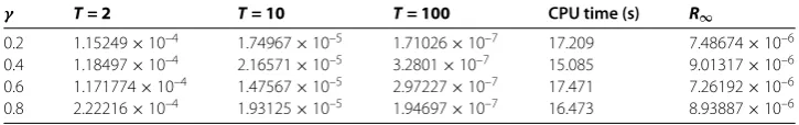
Table 1 The maximum absolute error withα= 1.4 for Example 9.1, the collocation method
γ T = 2 T = 10 T = 100 CPU time (s) R∞
0.2 1.15249×10⁻⁴ 1.74967×10⁻⁵ 1.71026×10⁻⁷ 17.209 7.48674×10⁻⁶ 0.4 1.18497×10⁻⁴ 2.16571×10⁻⁵ 3.2801×10⁻⁷ 15.085 9.01317×10⁻⁶ 0.6 1.171774×10⁻⁴ 1.47567×10⁻⁵ 2.97227×10⁻⁷ 17.471 7.26192×10⁻⁶ 0.8 2.22216×10⁻⁴ 1.93125×10⁻⁵ 1.94697×10⁻⁷ 16.473 8.93887×10⁻⁶
Table 2 The maximum absolute error withγ = 0.4 for Example 9.1, the Galerkin method
α T = 2 T = 10 T = 100 CPU time (s) R∞
1.2 1.18738×10⁻⁴ 2.17028×10⁻⁵ 2.28411×10⁻⁷ 17.082 5.4121×10⁻⁵
1.4 1.18497×10⁻⁴ 2.16751×10⁻⁵ 2.2801×10⁻⁷ 16.331 5.41498×10⁻⁵
1.6 1.18139×10⁻⁴ 2.15888×10⁻⁵ 2.27469×10⁻⁷ 16.472 5.42155×10⁻⁵ 1.8 1.17613×10⁻⁴ 2.14884×10⁻⁵ 2.26757×10⁻⁷ 16.256 5.43212×10⁻⁵
Initial and boundary conditions are
ρ(x),φ(x)w
s=
⇒ p[i, ] :=ρ(x),bi,(x)
ws=
k=
ρ(xk)bi,(xk)wk= , i= , , . . . , , ()
k(t),ψ(t)
wr=
⇒ p[k,j] :=k(t),Rj,n(t)
wr=
l=
k(tl)Rj,(tl)wl, k= , ,j= , , . . . , . ()
Finally, Eqs. ()-() give a system of equations, which can be solved for uij,i,j=
, , . . . , . Tables and show the maximum absolute error for collocation and Galerkin methods, respectively, forn= andβ= . and differentαandγ.
Example .([, ]) We consider the fractional diffusion equation () with the coeffi-cient functionsd(x,t) =(.)x.(whereis Euler’s gamma function),b(x,t) = (hence
γ = ) with the initial boundary conditions
u(x, ) =x( –x), u(,t) =u(,t) = .
Suppose that the exact solution isu(x,t) =x( –x)e–tfor suitable source term. The
Table 3 TheL∞error for Example 9.2 withα= 1.8 andβ= 1, the collocation method
n T = 2 T = 10 T = 100 CPU time (s) R∞
5 5.0×10⁻⁴ 2.5×10⁻⁵ 2.0×10⁻⁷ 4.37 7.82322×10⁻⁵
8 1.5×10⁻⁴ 1.5×10⁻⁴ 1.2×10⁻⁷ 12.917 3.52693×10⁻⁸
10 6.0×10⁻⁶ 6.0×10⁻⁶ 1.2×10⁻⁷ 21.669 1.60277×10⁻¹⁰
16 4.0×10⁻⁶ 3.0×10⁻⁶ 3.5×10⁻¹⁰ 74.458 2.32527×10⁻¹⁷
Table 4 TheL∞error for Example 9.2 withα= 1.8 andβ= 1, the Galerkin method
n T = 2 T = 10 T = 100 CPU time (s) R∞
5 3.0×10⁻³ 1.0×10⁻³ 5.0×10⁻⁴ 4.868 2.26905×10⁻³
8 8.0×10⁻⁴ 2.0×10⁻⁴ 5.0×10⁻⁵ 21.416 4.78888×10⁻⁶
10 1.5×10⁻⁴ 1.5×10⁻⁵ 1.2×10⁻⁵ 53.039 3.13802×10⁻⁸
16 1.5×10⁻⁶ 1.5×10⁻⁶ 8.0×10⁻⁷ 636.265 3.69793×10⁻¹⁵
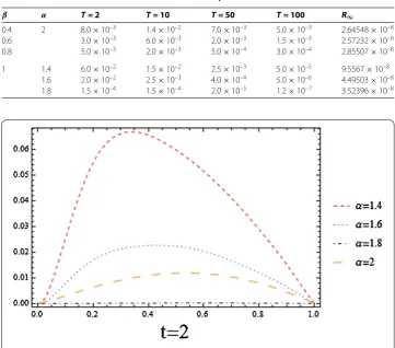
Table 5 Maximum residual errors forn= 8 for Example 9.2, the collocation method
β α T = 2 T = 10 T = 50 T = 100 R∞
0.4 2 8.0×10⁻³ 1.4×10⁻² 7.0×10⁻³ 5.0×10⁻³ 2.64548×10⁻⁸
0.6 3.0×10⁻³ 6.0×10⁻³ 2.0×10⁻³ 1.5×10⁻³ 2.57232×10⁻⁸
0.8 5.0×10⁻³ 2.0×10⁻³ 5.0×10⁻⁴ 3.0×10⁻⁴ 2.85507×10⁻⁸
1 1.4 6.0×10⁻² 1.5×10⁻² 2.5×10⁻³ 5.0×10⁻⁵ 9.5567×10⁻⁸
1.6 2.0×10⁻² 2.5×10⁻³ 4.0×10⁻⁴ 5.0×10⁻⁶ 4.49503×10⁻⁸
1.8 1.5×10⁻⁴ 1.5×10⁻⁴ 2.0×10⁻⁵ 1.2×10⁻⁷ 3.52396×10⁻⁸
Figure 1 The residual error for Example 9.2 withβ= 1 andn= 8 for differentα, and the collocation method fort= 2.
Example .([]) We consider the fractional diffusion equation () with the coefficient functionsd(x,t) =(.) x.,b(x,t) = (henceγ = ) with the initial boundary conditions
u(x, ) =x, u(,t) = , u(,t) =exp(–t).
Figure 2 The residual error for Example 9.2 withβ= 1 andn= 8 for differentα, and the collocation method fort= 10.
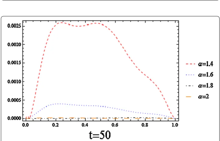
Figure 3 The residual error for Example 9.2 withβ= 1 andn= 8 for differentα, and the collocation method fort= 50.
Galerkin methods. Note that in these tables we provide CPU time (in seconds) consumed in the algorithms for obtaining the numerical solution, and when we compare these to-gether for one problem, we see the collocation method acting in a shorter time compared
with the Galerkin method. Table shows the maximum residual errors forn= when
Figure 4 The residual error for Example 9.2 withβ= 1 andn= 8 for differentα, and the collocation method fort= 100.
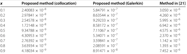
Table 6 The absolute error att= 1 withα= 1.8,β= 1 andn= 5 for Example 9.2
x Proposed method (collocation) Proposed method (Galerkin) Method in [21]
0.1 2.40083×10⁻⁸ 5.84791×10⁻⁷ 3.050×10⁻⁶
0.2 2.97841×10⁻⁸ 8.63544×10⁻⁷ 4.260×10⁻⁶
0.3 2.54578×10⁻⁸ 9.29233×10⁻⁷ 5.995×10⁻⁶
0.4 1.72148×10⁻⁸ 8.58172×10⁻⁷ 6.942×10⁻⁶
0.5 9.34788×10⁻⁹ 7.11067×10⁻⁷ 4.575×10⁻⁶
0.6 4.30953×10⁻⁹ 5.34071×10⁻⁷ 2.370×10⁻⁶
0.7 2.76392×10⁻⁹ 3.59841×10⁻⁷ 1.142×10⁻⁵
0.8 3.63934×10⁻⁹ 2.08591×10⁻⁷ 1.393×10⁻⁵
0.9 4.18034×10⁻⁹ 8.91471×10⁻⁸ 7.452×10⁻⁶
Table 7 TheL∞error for Example 9.3 withα= 1.8 andβ= 1, the collocation method
n T = 2 T = 10 T = 100 CPU time (s) R∞
5 4.0×10⁻³ 7.0×10⁻⁴ 1.2×10⁻⁵ 4.275 2.3301×10⁻⁴ 8 8.0×10⁻⁴ 1.0×10⁻³ 5.0×10⁻⁶ 13.009 8.91987×10⁻⁷ 10 6.0×10⁻⁵ 6.0×10⁻⁵ 4.0×10⁻⁷ 22.198 7.66056×10⁻⁹ 16 2.0×10⁻⁵ 2.0×10⁻⁵ 2.0×10⁻⁷ 76.581 9.82014×10⁻¹⁶
Table 8 TheL∞error for Example 9.3 withα= 1.8 andβ= 1, the Galerkin method
n T = 2 T = 10 T = 100 CPU time (s) R∞
5 1.5×10⁻² 7.0×10⁻³ 2.5×10⁻³ 5.053 1.267×10⁻³
8 8.0×10⁻³ 1.5×10⁻³ 7.0×10⁻⁴ 22.385 2.91652×10⁻⁶
10 2.5×10⁻³ 4.0×10⁻⁴ 3.0×10⁻⁴ 53.508 1.52719×10⁻⁸
16 1.4×10⁻⁵ 2.0×10⁻⁵ 6.0×10⁻⁶ 646.187 5.18714×10⁻¹⁶
Table 9 Maximum residual errors withn= 8 for Example 9.3, the Galerkin method
β α T = 2 T = 10 T = 50 T = 100 R∞
0.4 1.8 1.0×10⁻¹ 1.0×10⁻¹ 6.0×10⁻² 5.0×10⁻² 1.12744×10⁻⁷
0.6 8.0×10⁻² 6.0×10⁻² 2.5×10⁻² 2.5×10⁻² 3.93491×10⁻⁷
0.8 8.0×10⁻² 3.5×10⁻² 7.0×10⁻³ 1.0×10⁻² 1.60004×10⁻⁶
1 1.3 4.0×10⁻² 8.0×10⁻³ 2.0×10⁻³ 1.4×10⁻³ 1.36568×10⁻⁵
1.5 6.0×10⁻² 8.0×10⁻³ 4.0×10⁻³ 8.0×10⁻³ 2.85066×10⁻⁵
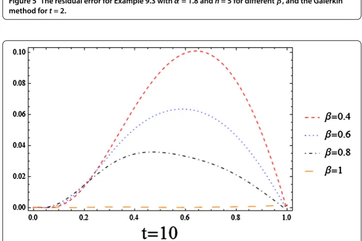
Figure 5 The residual error for Example 9.3 withα= 1.8 andn= 5 for differentβ, and the Galerkin method fort= 2.
Figure 6 The residual error for Example 9.3 withα= 1.8 andn= 5 for differentβ, and the Galerkin method fort= 10.
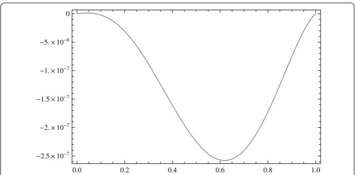
collocation method acting better than the method in []. Figures - show the abso-lute error att= forα= .,β= andn= in the intervalx∈[, ] in the collocation, Chebyshev spectral-Tau and Galerkin methods, respectively.
Example . We consider the fractional diffusion equation () with α= ., β = .,
γ = . and the coefficient functionsd(x,t) =t,b(x,t) =xand the source terms(x,t) such that the exact solution isu(x,t) =x( –x)exp(–t) +texp(–t) with the initial boundary conditions
Figure 7 The residual error for Example 9.3 withα= 1.8 andn= 5 for differentβ, and the Galerkin method fort= 50.
Figure 8 The residual error for Example 9.3 withα= 1.8 andn= 5 for differentβ, and the Galerkin method fort= 100.
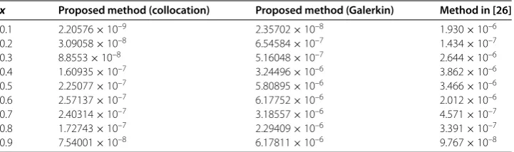
Table 10 The absolute error att= 1 withα= 1.8,β= 1 andn= 5 for Example 9.3
x Proposed method (collocation) Proposed method (Galerkin) Method in [26]
0.1 2.20576×10⁻⁹ 2.35702×10⁻⁸ 1.930×10⁻⁶
0.2 3.09058×10⁻⁸ 6.54584×10⁻⁷ 1.434×10⁻⁷
0.3 8.8553×10⁻⁸ 5.16048×10⁻⁷ 2.644×10⁻⁶
0.4 1.60935×10⁻⁷ 3.24496×10⁻⁶ 3.862×10⁻⁶
0.5 2.25077×10⁻⁷ 5.80895×10⁻⁶ 3.466×10⁻⁶
0.6 2.57137×10⁻⁷ 6.17752×10⁻⁶ 2.012×10⁻⁶
0.7 2.40314×10⁻⁷ 3.18557×10⁻⁶ 4.571×10⁻⁷
0.8 1.72743×10⁻⁷ 2.29409×10⁻⁶ 3.391×10⁻⁷
Figure 9 The absolute error att= 1 forα= 1.8,β= 1 andn= 5 in the interval 0 <x< 1 for Example 9.3 by the collocation method.
Figure 10 The absolute error att= 1 forα= 1.8,
β= 1 andn= 5 in the interval 0 <x< 1 for Example 9.3 by the method of [26].
Figure 11 The absolute error att= 1 forα= 1.8,β= 1 andn= 5 in the interval 0 <x< 1 for Example 9.3 by the Galerkin method.
Table 11 TheL∞error for Example 9.4, the collocation method
n T = 2 T = 10 T = 100 CPU time (s) R∞
5 4.0×10⁻³ 3.0×10⁻³ 2.0×10⁻⁷ 15.257 7.35512×10⁻³
8 7.0×10⁻⁴ 9.0×10⁻³ 7.0×10⁻⁸ 41.432 1.26371×10⁻⁶
10 1.0×10⁻³ 3.4×10⁻⁴ 4.0×10⁻⁹ 58.343 2.17796×10⁻⁹
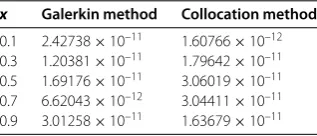
Table 12 The absolute error att= 1 andn= 8 for Example 9.4
x Galerkin method Collocation method
0.1 2.42738×10⁻¹¹ 1.60766×10⁻¹² 0.3 1.20381×10⁻¹¹ 1.79642×10⁻¹¹ 0.5 1.69176×10⁻¹¹ 3.06019×10⁻¹¹ 0.7 6.62043×10⁻¹² 3.04411×10⁻¹¹ 0.9 3.01258×10⁻¹¹ 1.63679×10⁻¹¹
The maximum errorsL∞for different values ofT andnare listed in Table for the
col-location method, and the results inx∈(, ) forn= are presented in Table att= for both methods.
10 Conclusion
In this article, we presented effective numerical methods for solving a space-time frac-tional diffusion equation with initial boundary conditions. For these problems defined in the unbounded time domain, we use the rational normalized Bernstein functions as basis functions to approximate the exact solution. We compared the execution of the colloca-tion and Galerkin methods using normalized Bernstein basis for solving a given problem. We have presented some numerical experiments to confirm the theoretical analysis. Pre-cision increases with the increase in the number of terms in the normalized Bernstein expansion. However, for the same number of terms, the collocation method yields rela-tively more accurate results in a compararela-tively shorter time compared with the Galerkin method. On the other hand, the collocation method is very sensitive to the collocation points. Generally, the most significant property of the collocation method is its fluency in the application; e.g., matrix elements of the given equation are evaluated directly rather than by numerical integration as in the Galerkin procedure. Generally, the results show that the proposed methods achieve better approximation accuracy than other methods, especially for the long time domain.
Acknowledgements
The authors would like to thank the referee for his valuable comments and suggestions which improved the paper into its present form.
Competing interests
The authors declare that they have no competing interests.
Authors’ contributions
Effective numerical methods for solving space-time fractional diffusion equation with initial boundary conditions are proposed. The rational normalized Bernstein functions as basis functions to approximate the exact solution are used in the unbounded time domain. Some numerical experiments to confirm the theoretical analysis are provided. In our examples we found that the collocation method yields relatively more accurate results in a comparatively shorter time compared with the Galerkin method; on the other hand, the collocation method is very sensitive to the collocation points. All authors read and approved the final manuscript.
Publisher’s Note
Springer Nature remains neutral with regard to jurisdictional claims in published maps and institutional affiliations.
Received: 26 June 2017 Accepted: 15 October 2017
References
1. Elwakil, AS: Fractional-order circuits and systems: an emerging interdisciplinary research area. IEEE Circuits Syst. Mag. 10(4), 40-50 (2010)
2. Xing, Y, Wu, X, Xu, Z: Multiclass least squares auto-correlation wavelet support vector machines. ICIC Express Lett. 2(4), 345-350 (2008)
4. Farouki, RT, Rajan, VT: Algorithms for polynomials in Bernstein form. Comput. Aided Geom. Des.5, 1-26 (1988) 5. Farouki, RT, Goodman, TNT: On the optimal stability of the Bernstein basis. Math. Comput.64, 1553-1566 (1996) 6. Alshbool, MHT, Bataineh, AS, Hashim, I, Isik, OR: Solution of fractional-order differential equations based on the
operational matrices of new fractional Bernstein functions. J. King Saud Univ., Sci.29(1), 1-18 (2017)
7. Alshbool, MHT, Hashim, I: Multistage Bernstein polynomials for the solutions of the fractional order stiff systems. J. King Saud Univ., Sci.28(4), 280-285 (2016)
8. Kemppainen, J: Existence and uniqueness of the solution for time-fractional diffusion equation with Robin boundary condition. Abstr. Appl. Anal.2011, Article ID 321903 (2011)
9. Podlubny, I: Fractional Differential Equations: An Introduction to Fractional Derivatives, Fractional Differential Equations, to Methods of Their Solution and Some of Their Applications, vol. 198. Academic Press, San Diego (1998) 10. Maleknejad, K, Basirat, B, Hashemizadeh, E: A Bernstein operational matrix approach for solving a system of high
order linear Volterra-Fredholm integro-differential equations. Math. Comput. Model.55, 1363-1372 (2012) 11. Akinlar, MA, Secer, A, Bayram, M: Numerical solution of fractional Benney equation. Appl. Math. Inf. Sci.8, 1-5 (2014) 12. Tadjeran, C, Meerschaert, MM, Scheffer, HP: A second-order accurate numerical approximation for the fractional
diffusion equation. J. Comput. Phys.213(1), 205-213 (2006)
13. Alipour, M, Rostamy, D, Baleanu, D: Solving multi-dimensional FOCPs with inequality constraint by BPs operational matrices. J. Vib. Control19(16), 2523-2540 (2013)
14. Bellucci, MA: On the explicit representation of orthonormal Bernstein polynomials, Department of Chemical Engineering, Massachusetts Institute of Technology, Cambridge, Massachusetts 02139, USA
15. Shen, J, Tang, T, Wang, L: Spectral Methods: Algorithms, Analysis and Applications. Springer, Berlin (2010) 16. Rostamy, D, Karimi, K: Bernstein polynomials for solving fractional heat-and wave-like equations. Fract. Calc. Appl.
Anal.15(4), 556-571 (2012)
17. Canuto, C, Hussaini, MY, Quarteroni, A, Zang, TA: Spectral Methods in Fluid Dynamic. Prentice Hall, Englewood Cliffs (1987)
18. Gottlieb, D, Hussaini, MY, Orszag, S: In: Voigt, R, Gottlieb, D, Hussaini, MY (eds.) Theory and Applications of Spectral Methods in Spectral Methods for Partial Differential Equations. SIAM, Philadelphia (1984)
19. Guo, BY, Shen, J, Wang, ZQ: Chebyshev rational spectral and pseudospectral methods on a semi-infinite interval. Int. J. Numer. Methods Eng.53, 65-84 (2000)
20. Ren, R, Li, H, Jiang, W, Song, M: An efficient Chebyshev-tau method for solving the space fractional diffusion equations. Appl. Math. Comput.224, 259-267 (2013)
21. Alavizadeh, SR, Maalek Ghaini, FM: Numerical solution of fractional diffusion equation over a long time domain. Appl. Math. Comput.263, 240-250 (2015)
22. Bhrawy, AH, Zaky, MA, Van Gorder, RA: A Space-Time Legendre Spectral Tau Method for the Two-Sided Space-Time Caputo Fractional Diffusion-Wave Equation. Springer, New York (2015)
23. Bass, RF: Real Analysis for Graduate Students, 2nd edn. (2011)
24. Bhrawy, AH, Zaky, MA: A method based on the Jacobi tau approximation for solving multi-term time-space fractional partial differential equations. J. Comput. Phys.281, 876-895 (2015)
25. Javadi, S, Babolian, E, Jani, M: A numerical scheme for space-time fractional advection-dispersion equation (2015). arXiv:1512.06629v1 [math.NA]