R E S E A R C H
Open Access
Mobility-dependent small-scale propagation
model for applied simulation studies
Dmitri Moltchanov
Abstract
We propose an extension to existing wireless channel modeling techniques introducing a notion of mobility behavior of the user. We represent large-scale propagation characteristics of wireless channels as a mobility-dependent stochastic process that explicitly tracks the movement of the user between areas with different received local average signal strength (RLASS). Our model consists of two different parts: mobility model and propagation model. Mobility of the user is modeled by a Markov chain with finite state space. Large-scale propagation characteristics of wireless channel are represented as a function of mobility model. Small-scale propagation characteristics are then obtained taking into account shadowing of the line-of-sight propagation path. Based on the amount of available information regarding a given landscape environment we develop two different parametrization methods (i) RLASS values are available for limited number of points in a given landscape and (ii) RLASS information is not available. The model is suitable for simulation studies of applications’ performance in presence of RLASS changes caused by movement of the user.
1 Introduction
To estimate performance of wireless channels propaga-tion models are often used. We distinguish between large-scale and small-scale models. The former models capture propagation characteristics on a coarse granular-ity using the notion of the received local average signal strength (RLASS), see e.g., [1-3]. Models characterizing rapid changes of the received signal strength are called small-scale propagation models, see e.g., [4-6]. These models capture propagation characteristics on a finer granularity.
Neither large-scale nor small-scale models take into account the signal strength attenuation caused by move-ments of a user. To be precise small-scale propagation models do take into account the so-called small-scale mobility of the user over short distances [7]. Such mod-els describe rapid fluctuations around a constant mean which are called fading. Such processes are implicitly assumed to be stationary at least in the second-order sense and mean equals to the received local average sig-nal strength (RLASS). However, if we would consider larger travel distances (i.e., more than just few meters) RLASS starts to vary and the most important factors
affecting it are terrain, speed of a mobile and distance from between transmitter and the receiver. In this arti-cle, contrarily to most small-scale propagation models proposed so far, we explicitly take into account two of these three factors–terrain and mobility of a user over it. In a mobile environment a user is allowed to change its position at any instant of time and these movements are not restricted to short travel distances. A receiver during a single session experiences different propagation characteristics. To predict these changes, an adequate model must capture both movement of a user between areas with different propagation characteristics and small-scale propagation characteristics in each area. Pro-pagation characteristics must be represented as a prob-abilistic function of user’s movements. Such model would be useful to estimate performance provided to applications while user is in traveling mode.
The rest of the article is organized as follows. In Sec-tion 2, we describe the structure of the model and intro-duce our modeling assumptions. Then, in Section 3, we propose three different parametrization methods for our model. Extensions and refinements of the model are dis-cussed in Section 4. Finally, in Section 5 we test some of our assumptions. Conclusions are provided in the last section.
Correspondence: [email protected]
Department of Communication Engineering, Tampere University of Technology, P.O. Box 553, Tampere, Finland
2 Structure of the model 2.1 Preliminary notes
The received signal strength in wireless networks is basically affected by three factors: (i) type of the terrain we consider (ii) speed of mobiles, and (iii) distance between the transmitter and receiver. Most small-scale propagation models proposed so far either implicitly or explicitly assumed that all these factors are fixed, i.e., a certain type of terrain is considered, speed of mobiles as well as distance between transmitter and receiver are fixed. The main reasons is that even with these assump-tions the resulting received signal strength is a covar-iance stationary stochastic process with complicated distributional and correlational properties. The reason for such reduced complexity of models is that small-scale propagation models were mainly used to design transceivers and associated lower layer techniques. For such tasks these models provide sufficient accuracy and should not be extended to more complex cases.
When performance of information transmission at higher layers is concerned we are interesting in adding those additional factors to the small-scale propagation models. Indeed, during the active session a mobile user may move inside and in-between cells experiencing not only qualitatively different propagation characteristics (e. g., different distributions but the same mean) but quan-titatively different too (e.g., different RLASS). Thus, in addition to the type of small-scale propagation at a cer-tain separation distance from the transmitter we also have to take into account movement of a user between areas with different RLASS. We would like to note that allowing at least one factor affecting the received signal strength to be variable may result in complex stochastic process making the model applicable for simulation stu-dies only.
2.2 The mobility model
Assume that a given cell of a circular shape is divided into a finite number of areas, M, such that these areas are non-overlapped and the sum of their areas equals to the area of the cell. Each area is associated with a cer-tain, not necessarily distinctive value of RLASS. We assume that a mobile user may probabilistically move between these areas.
Consider a discrete-time environment, i.e., time axis is slotted, the slot duration is constant and given by Δt. Changes of areas are only allowed at the slot boundaries. To capture movement of a user between areas we use a homogenous discrete-time Markov chain (DTMC) {SP (n), n= 0, 1, . . .}, SP(n)Î{1, 2, . . . , M}, whose states correspond to areas. LetDP be its transition probability
matrix. To parameterize this modelM, DP, andΔtshall be provided.
2.3 The large-scale propagation model
RLASS is mainly a function of the distance between the transmitter and the receiver and the type of propagation environment. To represent it, we associate a value of RLASS with each state of the mobility model. Let {P(n), n= 0, 1, . . .}, P(n) Î{P1, P2,. . . , PM} be the RLASS process whose underlying Markov chain is {SP(n), n= 0, 1, . . .}, i.e., the value of RLASS is modulated by the underlying Markov chain. To parameterize this model
we have to provide the RLASS vector
P= (P1,P2, ...,PM).
2.4 The small-scale propagation model
For performance evaluation studies, small-scale propaga-tion characteristics in a certain area can be modeled by doubly-stochastic process {Ri(n), n = 0, 1,. . .} modu-lated by homogenous DTMC {SR,i(n),n= 0, 1,. . .}, SR,
i(n)Î {1, 2, . . .,Hi}, each state of which is associated with conditional probability distribution function of the received signal strength FR,i(kΔf|j) (Δf) =Pr{Ri(n) =kΔf|
SR,i(n) =j},k= 1, 2,. . .,N,j= 1, 2,. . ., Hi, whereNis
the number of bins to which the signal strength is parti-tioned,Δfis the discretization interval. The slot duration
Δtof the model equals to the time to transmit a single bit at the wireless channel. Slot durations of mobility and small-scale propagation models are equal and synchronized.
To capture small-scale propagation characteristics we distinguish between LOS and NLOS environments. In the former case the small-scale propagation envelop dis-tribution is Rician. As the dominant component fades away the small-scale propagation envelop distribution degenerates to Rayleigh distribution. Thus, small-scale propagation characteristics in different areas are, at least, qualitatively (distribution) or quantitatively (RLASS) dif-ferent. Therefore, areas must be determined such that each of them is uniquely characterized by mean/distribu-tion pair. Then, each area must be associated with unique small-scale propagation model {Ri(n),n= 0, 1,. . .},i= 1,
2,. . .,Msuch thatE[Ri] =Pi, i.e., the RLASS in the area
iis the mean of {Ri(n),n= 0, 1,. . .}. We require that the state space of all small-scale propagation models is the same and given by {1, 2,. . .,H}.
slotn, i.e., {R(n), n= 0, 1, . . .} = {Ri(n),n= 0, 1,. . .}, SP (n) =i. Recalling that all small-scale propagation models were assumed to have the same number of states,H, the state-space of the resulting model is
SR(n)∈ {(1, 1), ..., (1,H), ..., (M, 1), ..., (M,H)}. (1)
An appropriate small-scale propagation model is only associated with the state of the mobility model corre-sponding to the appropriate area. Hence, transition probabilities of DTMC of mobility-dependent model is given by
dR,ij=dR,i,kj,k,j∈ {1, 2, ...,H},SP(n) =i. (2)
To parameterize mobility-dependent small-scale pro-pagation model we shall provideH, DR,i,FR,i(kΔf|j)(Δf),
i= 1, 2,. . .,M,k= 1, 2,. . ., N,j= 1, 2,. . .,H.
3 Parametrization of the model 3.1 The mobility model
Assume that the number of areas M and associated RLASS vector P are known. It is fair to expect MPthat the mean sojourn time in a certain area depends on its size. Consider a user that is in the area iin the slotn. In the next slot this user may stay in the areaior move to another area. The only areas to which a user can move in a slot are adjacent areas denoted byΩi. Con-sider areas fromΩias a single area. We compute transi-tion probability between areaiandΩias
dL,ii = between areaiand Ωi. Depending on the length of the border between area i and areas from Ωi transition probability dL,ii is distributed among transition prob-abilitiesdL,ij, jÎ Ωi, as
j. Parameterswij,jÎΩiare introduced to represent direc-tional movement of the user in a certain application sce-nario, e.g., highway, city center. Since this movement is specific for a given environment, no general expression can be provided. Note that j∈iwij = 1,i= 1, 2,. . .,M.
3.2 Large-scale propagation model
3.2.1 Parametrization based on measurements
Measurements of RLASS are often given by the 3D vec-tor PXY = (xi,yi,Pi), i = 1, 2, . . ., M, where M is the
number of measurements, (xi,yi) is the coordinate ofith measurement and Pi is the RLASS value of respective measurement.
Practically, it is not feasible to measure RLASS in each and every point of the landscape. Thus, information given by PXY is often insufficient to parameterize our
model. To estimate P and M we have to determine areas to which these measurements belong to, such that the approximation error is minimized. To determine areas we propose to use a division of the cell into areas whose vertexes are measurement points (xi, yi),i = 1, 2,
. . ., M. An appropriate division of the cell is given by
Voronoi (Dirichlet) tesselation separating a regionE of the spaceℜ2 into polygonsEi, i= 1, 2,. . ., M, usingM points drawn from a certain point process. In our case the space is ℜ2 and coordinates of measurements are considered as a realization of the point process. For each measurement point (xi, yi), Eiis the area consisting of all locations that are closer to (xi, yi) than to any other point. There are a number of algorithms to com-pute Voronoi tesselation [8].
To determine areas with different RLASS it is not strictly required to distinguish between values of RLASS in each area. Instead, it is possible to consider ranges of RLASS. In this case the range (max∀iPi-min∀iPi) must be divided intoKnon-overlapping ranges of length ΔP
= (max∀i Pi -min∀i Pi)/K. Then, all measurements are classified to these ranges. Adjacent areas having RLASS values falling in the same range can be grouped. An example is shown in Figure 1, where measurements points, the Voronoi tesselation, and resulting areas are shown.
3.2.2 Theoretical parametrization
Measurements of RLASS are often unavailable. In this case, we can parameterize our model based on approxi-mate estimation of shadowed areas and subsequent application of large-scale propagation models.
Assume that centers of shadowers are distributed according to the stationary Poisson point process with meanl. The parameter ldepends on a given landscape. Note that whenever possible actual placements of sha-dowers can be used. We also assume that (1) shasha-dowers are of rectangular form, (2) thickness of shadowers is zero, (3) their widths and heights are arbitrary distribu-ted, (4) height of the transmitter antennahais known.
outside, (3)ha< hs, the shadow virtually continues up to infinity. Since we consider a single cell, the latter two cases can be treated similarly.
The area of an arbitrary shadow is given by
Ss = min
4πR2 γ
360, 4π(d +ds)
2 γ
360
− dws
2 ,(5)
where
ds = min
hs
cotβ,R−d
,β = 90◦ −arctan d
ha −hs .
To estimate RLASS vector P we use large-scale pro-pagation models. It was shown in [9] that the mean value of propagation loss,L(d), can be approximated by
EL(d) = Ls (d0) + 10nlg
d d0
+ Xσ, (6)
whered is the separation distance,n is the path loss exponent,d0is the standard distance, Ls(d0) is the
pro-pagation loss at d0, Xsis the factor unique for a given
environment.
For every shadowed area the propagation loss is esti-mated using (6) withn >2, for unshad- owed areasn≈
2. Parameters for different frequency bands are given in [2,10]. Given a certain transmission power of the base station, propagation loss can be related to RLASS [7].
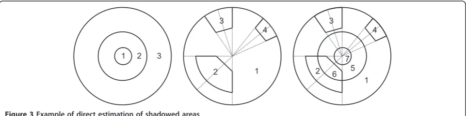
Observe that there can be shadows whose length is only slightly less than the radius of the cell. The range of RLASS corresponding to these shadows is large
leading to modeling errors. To avoid it, in addition to division of the cell into shadowed and non-shadowed areas, we propose to divide the cell into circles with dif-ferent radii. Shadows are then classified to these circles as shown in Figure 3.
Finally, we need to mention that performing theoreti-cal estimation of shadowed areas according to the pro-cedure described above there could be the case when two or more shadows overlap as shown in Figure 4, where different fillings denote doubly and triply over-lapped shadowed areas. In this case RLASS in the area where shadows overlap could be different compared to RLASS in non-overlapping regions of these areas. In this case the propagation loss in regions where two or more shadows overlap needs to be computed using different pass loss exponents.
3.3 The small-scale propagation model
We parameterize small-scale propagation models using the histogram matching method. Depending on pre-sence of LOS in the areai, process {Ri(n),n= 0, 1,. . .} has either Rician or Rayleigh distribution with mean E
[Ri] = Li. Setting the number of states of the Markov chain in each state of the mobility model to one (H= 1) and choosing Δfsmall enough we capture these distri-butions as
FR,i kf
f = pk
xk+1 − xk
. (7)
1 2
3 4
5
6 7 8 9 10
11 12
13
Figure 1Example of division of a cell based on measurements.
90o R 90o R R
ha>hs, ds<R-d ha>hs, ds>R-d ha<hs
ds ds ds
90o
d d
d
where pk =
xk+1
xk fX(x)dx,fX(x) is either Rayleigh or Rician distribution, xk and xk+1 are lower and upper
values for intervalk. Alternatively, settingHand solving the inverse-eigenvalue problem one can capture auto-correlation 1 and solving the inverse-eigenvalue problem one can capture autocorrelation properties of the received signal strength.
4 Extensions and notes 4.1 Signal-to-interference ratio
For a model to be useful, in addition to the received sig-nal strength we have to take into account the level of noise and consider the signal-to-interference (SI) ratio.
The interference at the receiver is given byI=W+U, whereWthe thermal noise, U= Ll=1U(l) is received signal strength fromL interfering base stations. W is usually assumed to be constant.Uis stochastic, depends on the distance and propagation path between the recei-ver and transmitters of interfering cells. Assume thatU
is constant for any state of the mobility model. The interference process {U(n),n= 0, 1,. . .},U(n) {U1,U2, .
. ., UM }, is modulated by {SP (n), n = 0, 1,. . .}. We determine the mean propagation loss E[L(mij)] for a given areaiand interfering transmitterjas a function of distance them,mij, using (6).E[L(mi)] is then related to RLASS and ‘mean other cells interference’is computed for areasias Ui = Ll=1Ui(l).
Adding a constantW to {U(n), n= 0, 1, . . .} affects the mean only allowing to consider the interference pro-cess {I(n), n= 0, 1,. . .}, i= 1, 2,. . .,M. The resulting signal-to-interference process is given by
Y(n) = ⎧ ⎨ ⎩
(R1 − I1) (n), SP (n) = 1,
. . . .
(RM − IM) (n),SP (n) = M,
(8)
where Ii = W +
L
l=1Ui (l),i = 1, 2, . . . ,M.
4.2 Attraction points
Notice that in our model movement of the user is homogenous in time and depends on the size of areas only, see (3). However, in addition to the size of the areas other factors may affect movement of the user of the landscape. One of the most important is the so-called attraction points in a cell, i.e., places (areas in our terminology) where a user may spent significant amount of time compared to other areas. Taking into account the effect of such attraction points is equivalent to intro-ducing non-homogeneity to the process of user move-ment between areas, that is, making movemove-ment to depend on some additional factors. Formally, it can be done introducing a new multipliers gi, i = 1, 2,. . ., M, each of which corresponds to a certain area into (3).
4.3 The scope of application
We would like to note that when micro or picocells sce-narios are considered the areas we introduced in this article are almost impossible to define. The reason is that in such cells attraction points seem to play much more important role compared to the size of areas. This is clearly seen considering “office” scenario, where employees move between pre-fixed locations such as working places, meeting rooms, etc. In this case instead of parameterizing our model based on sizes of areas we need to consider attractiveness of various locations and
7 6
1 2 3
2 3
4
1 2
3
4
1 5
Figure 3Example of direct estimation of shadowed areas.
inter-location movement of users developing new expressions for estimating inter-location movements. Since there could be a number of location-specific fac-tors involved into estimation of these probabilities we do not provide formulas for micro and picocells.
Our model was originally proposed for macrocell environments where it is possible to distinguish between different areas with quantitatively and/or qualitatively different received signal strength. The theoretical para-metrization of the model is suitable for suburbs and country-side areas. When measurements of RLASS are available the model can be applied in city-center scenar-ios. The only difference is that in addition to sizes of areas we also need to take into account possible tunnel-ing effects. Notice that even in this case we can use the-oretical parametrization. However, instead of propagation models specified in [1-3,10] we need to use special models suitable for such environment. Finally, as mentioned above with some modifications this model can be applied to microcell and picocell scenarios where a user moves between a number of attraction points. Applying this model in such scenarios additional care should be taken as even small travel distances may lead to drastic changes in small-scaled propagation character-istics due to complicated reflection and scattering observed in the buildings.
5 Testing assumptions
Unfortunately due to unavailability of data regarding mobility of users on the landscape we were not able to test closeness of the proposed mobility model and empirical data. Aside from this, one of the most impor-tant assumption we take in this article is that the received signal strength at a certain separation distance from the transmitter is indeed stationary while when changing the location different characteristics of the received signal strength distribution changes. To test this assumption we carried out experiments with wire-less local area network (WLAN) networks operating in infrastructure DCF mode according to IEEE 802.11b standard at 11 Mbps (DSSS) in laboratory environments. The access point is installed in the corridors with rooms along both sides of it. The main points of interest were characteristics of the received signal strength process at a certain separation distance from the transmitter and its changes as users move between different attraction points. Signal strength observations were measures with 1 ms granularity and then averaged over 0.5 ms time intervals.
To test our assumption regarding stationary nature if the received signal strength two rooms were arbitrarily chosen and the signal was measured for a long duration of time. Two samples gather as a result of these experi-ments are shown in Figure 5. Just observing these traces
no definitive conclusions regarding stationarity of the SNR process at a certain separation distance from the transmitter can be made. For this reason we performed detailed statistical analysis as discussed below.
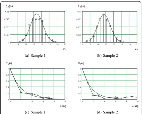
Histograms of relative frequencies service as estimates of empirical distributions and their approximations by Normal distribution are show in Figure 6. As one may observe approximations are quite good. Testing the null hypothesis about Normal distribution of data usingc2 test confirmed it with the level of significance,a, set to 0.1. Notice that for the second trace the null hypothesis is accepted even when a = 0.05. Tests performed for other rooms (not shown here due to space constraints) also confirm this approximation. We would like to note that one should not be surprised with normality of observations. Recall that we averaged the received signal strength over 0.5 s. intervals providing sufficient aggre-gation level for central limit theorem to hold.
In addition to distributional properties discussed above the process is found to be autocorrelated as high-lighted as normalized autocorrelation functions (NACF) shown in Figure 6c, d. The Ljung-Box test (a special type of portmanteau test) performed with the level of significance a= 0.1 showed that first three lags of the first sample and the first lag of the second one are sta-tistically different from zero with level of confidence a = 0.1. Observing the figures we see that the both func-tions decay geometrically fast.
Note that the above mentioned analysis does not allow us to conclude that the process at a certain separation distance is covariance stationary. Unfortunately, there are no well-behaved tests to access stationarity of sto-chastic processes. We use the following two-steps proce-dure. First of all, observe that explicitly assuming covariance stationarity the above mentioned analysis allows to model SNR data at a certain separation dis-tance from the transmitter using autoregressive process of order 1, AR(1), in the formYi=j0 +j1 Yi-1+εi,i=
by presence of correlation in subsamples. To conceal the effect of correlation we also used every second observa-tion in each subsample to compute empirical distribu-tions. The turning point test demonstrated that the hypothesis about white noise should be rejected with the level of significanta = 0.05 indicating that there is memory in each of those sample. Finally, in each sub-sample NACF decayed geometrically fast. The reason for performing the turning point test instead of, e.g., Ljung-Box portmanteau test is that it is unreasonable to expect the same number of lags having statistically sig-nificant correlation in samples of small sizes. Although these observations do not strictly prove that SNR pro-cess at a certain separation distance from the transmit-ter is covariance stationary they provide enough evidence that first and second-order characteristics likely remain unchanged.
Recall that in addition to covariance stationarity of SNR process as a certain separation distance from the
transmitter we also assumed that the mean (and possi-bly distribution) changes as user moves between differ-ent locations. To back up our assumption we performed the following experiments. A mobile station was in sta-tionary position for some noticeable amount of time. Then, a user moved into another office room and the station again remained in stationary state for some amount of time. Two arbitrarily chosen SNR samples obtained by changing the location of the user during the measuring process are shown in Figure 7. Observing these traces one may notice that the change in the received signal strength happens almost instantaneously. The reason is that the distances between attraction points in office environment are rather short (recall that the granularity of SNR measurements is 0.5 s).
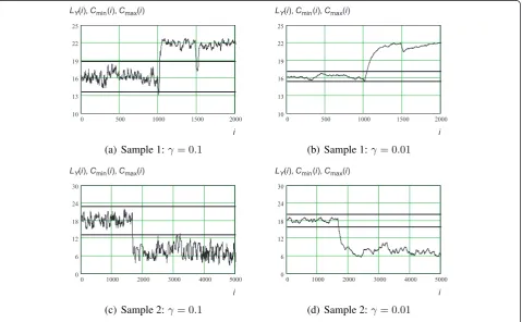
Results of EWMA change point test are shown in Fig-ure 8 for two values of smoothing parametersg. In all demonstrated figures the change in SNR statistics is detected. Moreover, our results show that changes are detected for all values of smoothing parametersg that are less than 0.1 implying that there is no need to access accuracy of the test using average run length (ARL) sta-tistics. Note that change-point statistical tests are rather coarse in general. To ensure that the change in some parameters of the distribution happened we compared distributional characteristics of two subsamples drawn from each sample. To get these subsamples we used results of EWMA test to exclude those observations occurring at the change point. c2 test performed with the level of significance set toa= 0.05 showed that the null hypothesis about the same empirical distribution should be rejected.
Note that the above mentioned statistical analysis demonstrate that (i) SNR process at a certain separation distance from the transmitter is close to covariance sta-tionary (ii) SNR process may quantitatively change when user changes its location. Supplementing the above mentioned analysis with mobility model between attrac-tion points we a particular case of the
mobility-Y(i)
0 500 1000 1500 2000 0
0 500 1000 1500 2000 0
Figure 5Samples of SNR observations (location is fixed).
fi,E(D)
dependent propagation model introduced in this article. Although these test have been performed in office envir-onment using IEEE 802.11b WLAN we can expect the same statistical behavior for public wireless networks. Still there are important differences. First of all, due to larger spaces covered by these networks in addition to attraction points we need to consider areas as described in Section 2. Secondly, changes in characteristics of the received signal strength are not expected to happen drastically as user moved between areas and/or attrac-tion points.
6 Conclusions
We developed an extension for wireless channel model-ing techniques explicitly takmodel-ing into account the move-ment of the user between areas with different small-scale propagation characteristics. Although a single cell environment has been considered, results can be extended to multiple cells scenario.
The model is suitable for performance evaluation of applications in presence of signal strength changes caused by movement of the user. Although the Markov structure of the model allows for analytical performance
Y(i)
0 1000 2000 3000 4000 5000 0
6 12 18 24 30
i
(a) Sample 1
Y(i)
0 500 1000 1500 2000 5
10 15 20 25 30
i
(b) Sample 2
Figure 7Time series of SNR observations (location is changed).
LY(i),Cmin(i),Cmax(i)
0 500 1000 1500 2000 10
13 16 19 22 25
i
(a) Sample 1:γ= 0.1
LY(i),Cmin(i),Cmax(i)
0 500 1000 1500 2000 10
13 16 19 22 25
i
(b) Sample 1:γ= 0.01
LY(i),Cmin(i),Cmax(i)
0 1000 2000 3000 4000 5000 0
6 12 18 24 30
i
(c) Sample 2:γ= 0.1
LY(i),Cmin(i),Cmax(i)
0 1000 2000 3000 4000 5000 0
6 12 18 24 30
i
(d) Sample 2:γ= 0.01
modeling, large state space may restrict its usage to simulation studies. We note that the model can be extended to capture propagation-dependent behavior. For example, the current modulation and coding scheme as a function of mobility of the user can be modeled.
Competing interests
The authors declare that they have no competing interests.
Received: 24 February 2011 Accepted: 2 April 2012 Published: 2 April 2012
References
1. T Okumura, E Omori, K Fakuda, Field strength and its variability in VHF and UHF land mobile service. Rev Electr Commun Lab.16(9/10):825–873 (1968) 2. M Hata, Empirical formula for propagation loss in land mobile radio
services. IEEE Trans Veh Tech.VT-29(3):317–325 (1980)
3. M Feuerestein, K Blackard, T Rappaport, S Seidel, H Xia, Path loss, delay spread, and outage models as functions of antena height for microcellular system design. IEEE Trans Veh Tech.43(3):487–498 (1994). doi:10.1109/ 25.312809
4. A Saleh, R Valenzuela, A statistical model for indoor multipath propagation. IEEE JSAC.5(2):128–137 (1987)
5. T Rappaport, Statistical channel impulse response models for factory and open plan building radio communication system design. IEEE Trans Commun.39(5):794–806 (1991). doi:10.1109/26.87142
6. D Durgin, T Rappaport, Theory of multipath shape factors for small-scale fading wireless channels. IEEE Trans Ant Propag.48, 682–693 (2000). doi:10.1109/8.855486
7. T Rappaport,Wireless Communications: Principles and Practice, 2nd edn. (Prentice Hall, Upper Saddle River, 2002)
8. P Green, R Sibson, Computing Dirichlet tesselations in the plane. Comput J.
21, 168–173 (1978)
9. S Seidel, Path loss, scattering and multipath delay statistics in four european cities of digital cellular and microcellular radiotelephone. IEEE Trans Veh Tech.40(4):721–730 (1991). doi:10.1109/25.108383
10. Digital mobile radio, towards future generation systems. COST 231 Final Report, EUR18957. (1999)
11. D Moltchanov, State description of wireless channels using change-point statistical tests. in Proc WWIC’2006, vol. 3970. (Bern, Switzerland, 2006), pp. 275–286
12. W Schmid, A Schone, Some properties of the EWMA control chart in the presence of auto-correlation. Ann Stat.25(3):1277–1283 (1997). doi:10.1214/ aos/1069362748
doi:10.1186/1687-1499-2012-130
Cite this article as:Moltchanov:Mobility-dependent small-scale propagation model for applied simulation studies.EURASIP Journal on Wireless Communications and Networking20122012:130.
Submit your manuscript to a
journal and benefi t from:
7 Convenient online submission 7 Rigorous peer review
7 Immediate publication on acceptance 7 Open access: articles freely available online 7 High visibility within the fi eld
7 Retaining the copyright to your article