A new parallel difference algorithm based on improved alternating segment Crank–Nicolson scheme for time fractional reaction–diffusion equation

R E S E A R C H

Open Access

A new parallel difference algorithm based on

improved alternating segment

Crank–Nicolson scheme for time fractional

reaction–diffusion equation

Xiaozhong Yang

_{and Xu Dang}

*_{Correspondence:}

[email protected] 1_{School of Mathematics and}

Physics, North China Electric Power University, Beijing, China

Abstract

The fractional reaction–diffusion equation has profound physical and engineering background, and its rapid solution research is of important scientific significance and engineering application value. In this paper, we propose a parallel computing method of mixed difference scheme for time fractional reaction–diffusion equation and construct a class of improved alternating segment Crank–Nicolson (IASC–N) difference schemes. The class of parallel difference schemes constructed in this paper, based on the classical Crank–Nicolson (C–N) scheme and classical explicit and implicit schemes, combines with alternating segment techniques. We illustrate the unique existence, unconditional stability, and convergence of the parallel difference scheme solution theoretically. Numerical experiments verify the theoretical analysis, which shows that the IASC–N scheme has second order spatial accuracy and 2 –

α

computation accuracy and obvious parallel computing properties, showing that the IASC–N parallel difference method is effective for solving time fractional

reaction–diffusion equation.

MSC: 65M06; 65M12; 65Y05

Keywords: Fractional reaction–diffusion equation; IASC–N difference scheme; Unconditional stability; Order of convergence; Parallel computing

1 Introduction

The fractional reaction–diffusion equation has a profound physical background and rich theoretical connotation. As the application of fractional calculus increases, the solution of fractional evolution equation has become an urgent research work (Baleanu et al. 2018; Mohammadi et al. 2018; Hajipour et al. 2019; Baleanu et al. 2019) [1–4]. The analytical solution of fractional reaction–diffusion equation is difficult to give explicitly. Even the analytical solution of linear fractional reaction–diffusion equation mostly contains special functions, such as Mittag-Leffler functions (Kumar et al. 2018; Kumar et al. 2018; Singh et al. 2019) [5–7]. The series corresponding to these functions converge slowly, and the calculation of these special functions is quite difficult in practical applications. Therefore,

all mentioned above make the high-efficiency numerical simulation of fractional reaction– diffusion equation an urgent research problem (Uchaikin 2013; Chen et al. 2010) [8,9]. Since fractional calculus has historical dependence and global correlation, the amount of computation and storage of numerical simulation for fractional differential equation is extremely large. Even with high-performance computers, it is difficult to simulate in long-term history (the amount of computation increases exponentially with the increase of time) or large computational domain (Guo et al. 2015; Sabatier et al. 2014) [10,11]. Starting from the urgent need of scientific engineering computing in the era of big data, the finite difference parallel computing method for fractional reaction–diffusion equation has important scientific significance and engineering application value.

For the numerical computation of fractional evolution equation, more and more numer-ical computation methods are proposed (Singh et al. 2018; Kumar et al. 2018; Goswami et al. 2019) [12–14]. At present, the relatively more mature methods are still the finite dif-ference method and the series method (mainly Adomian decomposition and variational iterative method). Among them, the finite difference method has a wide application range. The advantages of the finite difference method are reflected in solving problems in small spatial domain and short time history. The accuracy and stability of the algorithm can meet the needs of numerical simulation of small-scale problems (Sun and Gao 2015; Liu et al. 2015) [15,16]. The theoretical analysis methods mainly include Fourier method, energy estimation, matrix method (eigenvalue), mathematical induction, and some other numer-ical methods, but most of them cannot be used as universal numernumer-ical methods or lack a perfect theoretical analysis. For time fractional diffusion equation, Lin and Xu (2007) [17] constructed a finite difference scheme in time domain and a Legendre spectrum method in spatial domain and proved the unconditional stability and convergence of the method. For time fractional fourth order reaction–diffusion equation with nonlinear reaction term, Liu et al. (2015) [18] proposed a finite difference approximation in time direction and a finite element approximation in spatial direction to obtain the numerical solution of the time fractional fourth order reaction–diffusion equation and analyzed the unconditional stability of the method. For time fractional reaction–diffusion equation, Liu et al. (2015) [19] proposed anH1_{-Galerkin mixed finite element method and obtained the numerical} results with optimal time and spatial convergence order. Chen et al. (2016) [20] discussed the numerical solution of distribution order time fractional reaction–diffusion equation in semi-infinite spatial domain and proposed a fully discrete scheme based on finite differ-ence method in time domain and spectral approximation using Laguerre function in spa-tial domain. The numerical experiments verified the effectiveness of the proposed scheme. Zhang and Yang (2018) [21] gave a class of explicit–implicit (E–I) and implicit–explicit (I– E) difference methods for time fractional reaction–diffusion equation. The method had second order spatial precision and 2 –αorder time precision, and its computation time was nearly 41% lower than that of the classical implicit difference scheme.

gener-ally has good stability but is not suitable for parallelization. Inspired by the method of con-structing AGE scheme, Zhang et al. (1994) [25] proposed the idea of constructing segment implicit schemes using Saul’yev asymmetric scheme, and appropriately used alternating techniques to establish a variety of explicit–implicit and pure implicit alternating parallel methods, which obtained research results with both stability and parallelism. Academi-cian Zhou (1997) [26] called the mixed explicit and implicit schemes for the most general parabolic equation as a difference scheme with intrinsic parallelism. He studied the theo-retical issues such as the existence, uniqueness, convergence, and stability of the difference decomposition, and established the basic theory of the difference methods with intrinsic parallelism for parabolic equation. Wang (2006) [27] constructed a class of alternating dif-ference schemes with intrinsic parallelism for the KdV equation using Saul’yev asymmetric scheme combined with C–N difference scheme and proved the linear absolute stability of the scheme. Yuan et al. (2007) [28] proposed a class of parallel difference schemes with unconditional stability and second order spatial precision for nonlinear parabolic equa-tion. The main advantage of these difference schemes with intrinsic parallelism is that the schemes can be directly applied to parallel computer systems with distributed memory and minimize the amounts of communication between processors. The algorithm only needs to transfer local messages between adjacent processors. The communication and computation involved are local so that it is easier to load balance between them, thus ob-taining good precision and scalability of parallel computing.

communi-cation, properly allocating computational tasks, and trying not to change the original serial difference scheme. Wu et al. (2018) [37] proposed an alternating segment Crank–Nicolson parallel difference scheme for time fractional sub-diffusion equation, which had ideal com-puting accuracy and efficiency. For nonlinear time-space fractional parabolic partial differ-ential equations, Biala and Khaliq (2018) [38] developed a time stepping scheme which was implemented in parallel using the distributed (MPI), shared memory systems (OpenMP), and a combination of both, and the scheme was shown to be convergent and of order 1 +α. Fu and Wang (2019) [39] developed a fast parallel finite difference method for space-time fractional partial differential equations, which used a matrix-free preconditioned fast Krylov subspace iterative solver at each time step, significantly reducing computational complexity and memory requirement.

We do not study parallel algorithms from the perspective of numerical algebra, but based on the parallelization of traditional differential schemes, we seek to explore another way of parallelization skipping the difficulty of numerical algebra. A class of mixed differ-ence parallel computing methods for solving fractional reaction–diffusion equation is pro-posed in this paper. Based on the classical C–N scheme and classical explicit and implicit schemes, our proposed method combines alternating segment techniques to construct an improved alternating segment Crank–Nicolson (IASC–N) difference scheme. We an-alyze the existence, uniqueness, unconditional stability, and convergence of the IASC–N scheme solution theoretically, and numerical experiments verify the theoretical analysis. The computational efficiency of IASC–N scheme is greatly improved compared to the im-plicit scheme and the C–N scheme. The ideal computational accuracy and obvious parallel computing properties indicate that the IASC–N parallel difference scheme is effective for solving time fractional reaction–diffusion equation.

The structure of this paper is as follows. In Sect.2, the time fractional reaction–diffusion equation is given and the IASC–N parallel difference scheme is constructed. In Sect.3, the unique solvability, stability, and convergence of the method are proved rigorously. In Sect.4, the specific numerical example is given which verifies the efficiency of the con-structed scheme and supports theoretical results.

2 Alternating segment C–N parallel difference scheme for time fractional reaction–diffusion equation

2.1 Time fractional reaction–diffusion equation

Consider the time fractional reaction–diffusion equation defined in regionΩ={0≤x≤ L, 0≤t≤T}(Uchaikin 2013; Chen et al. 2010; Guo et al. 2015) [8–10]:

⎧ ⎪ ⎪ ⎨ ⎪ ⎪ ⎩

∂αu(x,t)

∂tα =

∂2u(x,t)

∂x2 –pu(x,t) +f(x,t),

u(x, 0) =u0(x),

u(0,t) =u(L,t) = 0,

(1)

where f(x,t) andu0(x) are given functions,pis a nonnegative constant, 0 <α< 1, and

∂αu(x,t)

∂tα is a Caputo-type fractional derivative defined by

C

0D

α

tu(x,t) =

∂α_u(x,t)

∂tα =

1

Γ(1 –α)

t

0

∂u(x,ξ)

∂ξ

dξ

Whenf(x,t) = 0, the analytical solution of Eq. (1) in regionΩ={0≤x≤L, 0≤t≤T}

can be obtained by finite sine and Laplace transforms as follows (Guo et al. 2015; Sabatier et al. 2014) [10,11]:

2.2 A class of IASC–N parallel difference schemes

With the space stephand the time stepτ, the solution regionΩ is divided into grids and the grid points are (xi,tk). Let space step h= _ML and time stepτ = T_N, thenxi=ih,

i= 0, 1, 2, . . . ,M, andtk=kτ,k= 0, 1, 2, . . . ,N. LetUikbe the numerical solution tou(xi,tk)

andfk

i be the exact solution tof(xi,tk).

The time fractional derivative of Eq. (1) can be discretized into the following form:

∂α_u(x

To construct the IASC–N scheme of Eq. (1), give the following three discrete schemes first, wherec=τα_{Γ(2 –α),a=} c

h2, andb=pc. (1) Classical explicit difference scheme

C

In conjunction with Eq. (2), the above scheme can be rewritten as

k

(2) Classical implicit difference scheme

In conjunction with Eq. (2), the above scheme can be rewritten as

In conjunction with Eq. (2), the above scheme can be rewritten as

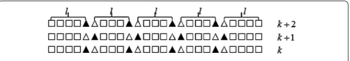
Figure 1Schematic diagram of the IASC–N scheme (B= 5)

and calculate the inner points by the C–N scheme (8). For points on even time layers, wheni0=l, 2l, . . . , (B– 1)l, calculate the inner boundary points (xi0,tk+2) by the classical implicit scheme (7); wheni0=l+ 1, 2l+ 1, . . . , (B– 1)l+ 1, calculate the inner boundary points (xi0,tk+2) by the classical explicit scheme (6); and calculate the inner points by the C–N scheme (8). Particularly, use the C–N scheme at the boundary of both ends of the time numerical layers.

LetM= 26,B= 5, andl= 5. The construction principle of IASC–N scheme is shown in Fig.1, where the classical explicit scheme is used inplace, the classical implicit scheme is used inplace, and the C–N scheme is used inplace.

Above all, the IASC–N scheme of Eq. (1) can be constructed as follows:

3 Numerical analysis of IASC–N scheme for time fractional reaction–diffusion equation

3.1 Existence and uniqueness of IASC–N scheme solution Since

is a weak diagonally dominant matrix,I+A1Gis a strict diagonally dominant matrix. Similarly,I+A2Gis also a strict diagonally dominant matrix. We have that the coefficient matricesI+A1GandI+A2Gof IASC–N scheme (9) are non-singular matrices. So there is the following theorem.

Theorem 1 The IASC–N parallel difference scheme (9) for time fractional reaction–

diffusion equation has a unique solution.

3.2 Unconditional stability of IASC–N scheme

Lemma 1(Kellogg lemma [27]) If matrix A+AT_{is nonnegative,then for∀θ> 0,there is}

is a weak diagonally dominant matrix and the diagonal elements are nonnegative real num-bers,A1G+ (A1G)Tis a nonnegative definite matrix. Similarly,A2G+ (A2G)Tis also a

non-negative definite matrix. The lemma is proved.

It is easy to get that the minimum eigenvalues of the matricesA1GandA2Gare zero. Letλ1andλ2(λ1,λ2≥0) be any eigenvalue of the matrixA1G, there is(c1I–A1G)(c1I+

A1G)–12=max{|c_c1₁–₊λλ12|} ≤1 by Lemma1and Lemma2. Therefore, letλ2= 0 andλ1be taken as the eigenvalue of the matrix A1G, which makes |c1–λ1|the largest, we have

|c1–λ1|

c1+λ2 ≤1. Letλ3andλ4 (λ3,λ4≥0) be any eigenvalue of the matrixA2G. Obtained by (c1I–A2G)(c1I+A2G)–12=max{|_cc1₁–_+λλ3₄|} ≤1, letλ4= 0 andλ3be taken as the eigenvalue of the matrixA2G, which makes|c1–λ3|the largest, we get|_cc1₁–₊λλ43|≤1.

When 0≤λ1≤c1, we have |c1₁₊–λλ1|+4l1 =

c1–λ1+l1

1+λ4 = 1 –λ1≤1.

Whenλ1>c1, letλ1=r1c1(r1> 1), from|c_c1₁₊–λλ12|≤1,r1≤2 can be obtained. Therefore, there isc1<λ1≤2c1, and|c1–₁₊λλ1|+4l1 =

λ1–c1+l1 1+λ4 ≤

2c1–c1+l1

1+λ4 = 1 at this time. Above all, |c1–λ1|+l1

1+λ4 ≤1. Similarly, we can get

|c1–λ3|+l1 1+λ2 ≤1. Whenk= 1 (kis the time layer),

E1₂ =(I+G1)–1(I–G2)E0₂

≤(I+G1)–1₂(I–G2)E0₂

≤|1 –λ3| 1 +λ2

E0₂

≤E0₂.

Whenk= 2,

E2₂ =(I+G2)–1

(c1I–G1)E1+l1E0₂

≤(I+G2)–1₂(c1I–G1)E1+l1E0₂

≤|c1–λ1|+l1 1 +λ4

E0₂

≤E0₂.

It is assumed that whenk≤2n,Ek2≤ E02holds. Then there are

E2n+1₂=(I+G1)–1

(c1I–G2)E2n+c2E2n–1+· · ·+c2nE1+l2nE0₂

≤(I+G1)–1₂(c1I–G2)E2n+c2E2n–1+· · ·+c2nE1+l2nE0₂

≤|c1–λ3|+c2+· · ·+c2n+l2n

1 +λ2

E0₂

=|c1–λ3|+l1 1 +λ2

E0₂

≤E0₂,

E2n+2₂=(I+G2)–1(c1I–G1)E2n+1+c2E2n+· · ·+c2n+1E1+l2n+1E0₂ ≤(I+G2)–1₂(c1I–G1)E2n+1+c2E2n+· · ·+c2n+1E1+l2n+1E0₂

≤|c1–λ1|+c2+· · ·+c2n+1+l2n+1 1 +λ4

E0₂

=|c1–λ1|+l1 1 +λ4

E0₂

Above all, we can getEk_{2≤ E}0_{2, wherek= 1, 2, . . . ,N.}

Theorem 2 The IASC–N parallel difference scheme (9) for time fractional reaction–

diffusion equation is unconditionally stable.

3.3 Convergence of IASC–N scheme It is known thatC

Consider the explicit scheme (10) onk+ 1 time layer and the implicit scheme (11) on

k+ 2 time layer:

Consider C–N scheme (12) onk+ 1 time layer and C–N scheme (13) onk+ 2 time layer:

Perform the Taylor expansion of schemes (12) and (13) atU_ik+1respectively, and obtain the truncation errorsT3(τ,h) andT4(τ,h) as follows:

When explicit and implicit schemes are used alternately in different time layers, the τUxxt andpτUt terms in the truncation errors T1(τ,h) and T2(τ,h) are canceled. schemes are used alternately in different time layers, the τ

2Uxxt and

pτ

2Ut terms of the truncation errorsT3(τ,h) andT4(τ,h) are canceled. So the scheme accuracy at the inner points and the boundary at both ends is stillO(τ2–α_+h2_).

Theorem 3 The computation accuracy of the IASC–N parallel difference scheme(9)for

time fractional reaction–diffusion equation is O(τ2–α_+h2_).

4 Numerical experiments

The numerical experiments are based on Intel Core i5-3230 CPU and run in Mat-labR2016a environment (Liu 2012) [42]. We consider the following fractional reaction– diffusion equation (Lin and Xu 2007; Jiang and Ma 2011) [17,43]:

wheref(x,t) =_Γ(3–2_α)t2–α_{sin(2πx) + 4π}2_t2_{sin(2πx),u0(x) = 0,p= 0, and 0 <α< 1. It is easy} to get its analytical solution as follows (Lin and Xu 2007; Jiang and Ma 2011) [17,43]:

u(x,t) =t2sin(2πx). (15)

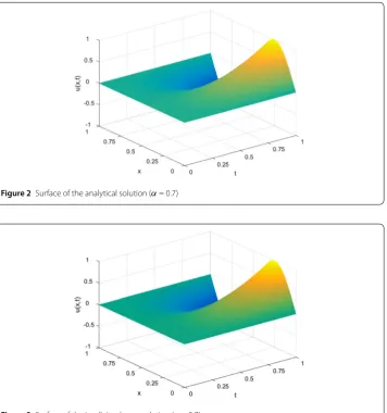
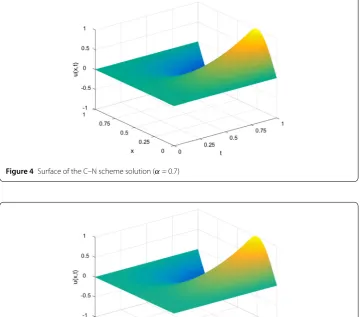
Takeα= 0.7,M= 81,N= 1000,B= 5, andl=M_B–1= 16, and give surface plots of the ana-lytical solution (15), implicit scheme solution, C–N scheme solution, and IASC–N scheme solution (9) as follows. As can be seen from Fig.2, Fig.3, Fig.4, and Fig.5, the shape of the three scheme solution surfaces is consistent with the shape of the analytical solution surface, and the surface of the IASC–N scheme solution is smooth.

Lett= 0.4, and compare the IASC–N scheme solution, implicit scheme solution, and C–N scheme solution with the analytical solution. The scheme solution is very close to the analytical solution. The computation results are shown in Table1.

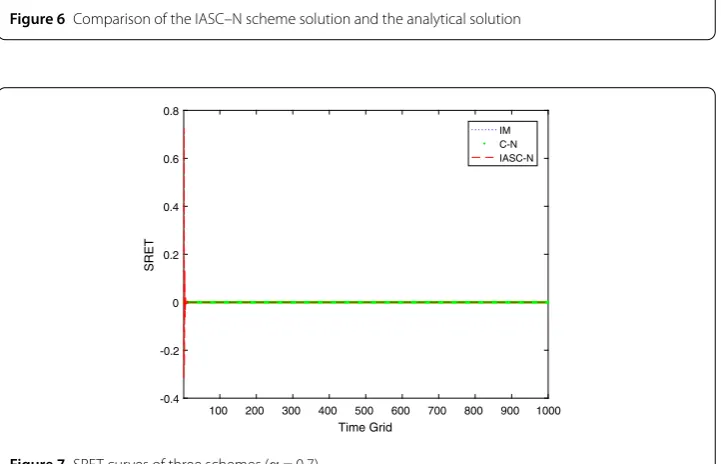
Takeα= 0.3, 0.5, 0.7 respectively, and compare the scheme solutions with the analytical solutions att= 0.4. The computation result is shown in Fig.6. The scheme solution curve is very close to the analytical solution curve, indicating that the fractional order parameter

αhas little effect on the computation accuracy, that is, the fractional order does not have

Figure 2Surface of the analytical solution (α= 0.7)

Figure 4Surface of the C–N scheme solution (α= 0.7)

Figure 5Surface of the IASC–N scheme solution (α= 0.7)

Table 1 Comparison of scheme solutions and analytical solutions (α= 0.7)

x 0.2 0.4 0.6 0.8

Analytical solution 0.152169 0.094046 –0.094046 –0.152169 Implicit scheme solution 0.152168 0.094023 –0.094023 –0.152168 C–N scheme solution 0.152184 0.094011 –0.094011 –0.152184 IASC–N scheme solution 0.151216 0.087818 –0.087822 –0.151209

much influence on the dynamic behavior of the system. Therefore, the IASC–N method is a high precision difference method for solving fractional reaction–diffusion equation.

In order to verify the stability and computation accuracy of the IASC–N scheme, take

α= 0.7,M= 81, andN= 1000, and give the change of relative error with time and space changing. Let the equation analytical solutionuk_i be the control solution and the scheme solutionU_ik be the disturbance solution. The sum of relative error for every time level (SRET) and the difference total energy (DTE) are defined as follows:

SRET(k) =

M

i=1 |uk

i –Uik|

Uk i

, DTE(i) = 1 2

N

k=1

Figure 6Comparison of the IASC–N scheme solution and the analytical solution

Figure 7SRET curves of three schemes (α= 0.7)

The SRET curve in Fig.7shows that although the error of the scheme solution is slightly larger when the number of time layers is small, as the number of time layers increases, SRET decreases rapidly and tends to zero, indicating that the IASC–N scheme for time fractional reaction–diffusion equation is computationally stable.

The DTE curve in Fig.8shows that the IASC–N scheme solution better approximates the analytical solution compared to the implicit scheme solution and the C–N scheme solution. The DTE curves of the three schemes have similar trends and are all less than 2.5×10–5_{, indicating that the IASC–N scheme for time fractional reaction–diffusion} equation has good computational accuracy.

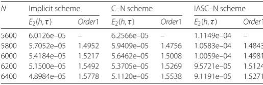
The time convergence order and spatial convergence order of the IASC–N scheme are verified below. DefineE2(h,τ) as theL2_{mode,Order1 as the time convergence order, and}

Order2 as the spatial convergence order as follows (Jiang and Ma 2011) [43]:

E2(h,τ) = max 0≤k≤N

Figure 8DTE curves of three schemes (α= 0.7)

Table 2 Scheme errors and time convergence orders (α= 0.5,h=₈₀1)

N Implicit scheme C–N scheme IASC–N scheme

E2(h,τ) Order1 E2(h,τ) Order1 E2(h,τ) Order1

5600 6.0126e–05 – 6.2566e–05 – 1.1149e–04 –

5800 5.7052e–05 1.4952 5.9409e–05 1.4756 1.0583e–04 1.4843

6000 5.4184e–05 1.5217 5.6462e–05 1.5008 1.0059e–04 1.4981

6200 5.1500e–05 1.5492 5.3705e–05 1.5269 9.5721e–05 1.5124

6400 4.8984e–05 1.5778 5.1120e–05 1.5538 9.1191e–05 1.5271

Table 3 Scheme errors and spatial convergence orders (α= 0.5,τ=h2)

M Implicit scheme C–N scheme IASC–N scheme

E2(h,τ) Order2 E2(h,τ) Order2 E2(h,τ) Order2

101 3.2314e–04 – 3.3097e–04 – 6.2148e–04 –

201 8.0660e–05 2.0167 8.2618e–05 2.0166 1.5433e–04 2.0242

301 3.5826e–05 2.0098 3.6697e–05 2.0097 6.8421e–05 2.0144

401 2.0146e–05 2.0070 2.0635e–05 2.0069 3.8438e–05 2.0103

501 1.2891e–05 2.0054 1.3204e–05 2.0054 2.4571e–05 2.0097

Order1 =ln(

E2(h,τ1)

E2(h,τ2))

ln(τ1

τ2)

, Order2 =ln(

E2(h1,τ)

E2(h2,τ))

ln(h1

h2) .

Takeα= 0.5 andN= 5600, 5800, 6000, 6200, 6400, and leth=₈₀1, that is, takeM= 81. The computation results of the time convergence order are shown in Table2. The accuracy of IASC–N scheme is close to 2 –αorder in time, which is consistent with the IASC–N scheme accuracy ofO(τ2–α_+h2_{) in the theoretical analysis.}

Takeα= 0.5 andM= 101, 201, 301, 401, 501, and letτ=h2, that is, takeN≈ M₄2. The computation results of the spatial convergence order are shown in Table3. The accuracy of IASC–N scheme is spatially close to 2 order, which is similar to the error of the implicit scheme and the C–N scheme.

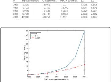
Table 4 Computing time and speedup of scheme solution (α= 0.7)

M Implicit scheme/s C–N scheme/s IASC–N scheme/s Sp1 Sp2

3001 2.3513 2.5916 1.9731 1.1916 1.3135

4001 5.1555 5.3499 3.6795 1.4011 1.4540

5001 8.9145 9.1686 5.7039 1.5629 1.6074

6001 19.7645 20.4187 8.5569 2.3098 2.3862

7001 48.9845 49.8756 11.5971 4.2238 4.3007

Figure 9Comparison of computing time between the three schemes (α= 0.7)

N scheme relative to the implicit scheme, andSp2is the the speedup of IASC–N scheme relative to the C–N scheme.

Table4shows that the computing time of IASC–N scheme is much smaller than that of the implicit scheme and C–N scheme, and as the number of spatial grids increases,Sp1 andSp2also increase, indicating that the computing time growth rate of IASC–N scheme is smaller than the computing time growth rate of the implicit scheme and C–N scheme. It is valid to verify that the IASC–N scheme for time fractional reaction–diffusion equation is effective.

In order to more clearly compare the computational efficiency of IASC–N scheme, im-plicit scheme, and C–N scheme, takeα= 0.7 andN= 100, and give the variation of the computing time of the three schemes with the increase of the number of spatial grids as Fig.9.

5 Conclusions

For a long time, a large number of parallel schemes have been designed to be condition-ally stable or unconditioncondition-ally stable but with only first order spatial accuracy (Yuan et al. 2015) [45]. In order to obtain the parallel difference scheme with higher accuracy and looser stability condition, this paper proposes a parallel computing method of IASC–N difference scheme for time fractional reaction–diffusion equation. Theoretically, we ana-lyze the unique solvability, unconditional stability, convergence, second order spatial ac-curacy, and 2 –αorder temporal accuracy of the IASC–N scheme. Numerical experiments verify the theoretical analysis, indicating that the proposed IASC–N difference scheme is more accurate and efficient than that given in [17,43]. In particular, when the number of spatial grids is large enough, the IASC–N method has obvious localization features in terms of computation and communication and is suitable for operating in massive parallel computing systems. The parallel computing method of IASC–N difference scheme in this paper can be extended to high dimensional equations to solve the numerical solution of high dimensional fractional reaction–diffusion problems. We will also consider more nu-merical methods (Hajipour et al. 2018; Hajipour et al. 2018) [46,47] applying to numerical solutions for other fractional evolution equations.

Acknowledgements

The authors would like to deeply thank Dr. Lifei Wu (School of Mathematics and Physics, North China Electric Power University) for his valuable suggestion and constructive comments during the preparation.

Funding

The research is supported by the National Natural Science Foundation of China (Grant No. 11371135) and the National Major Scientific and Technological Special Project (Grant No. 2017ZX07101001-01).

Competing interests

The authors declare that they have no competing interests.

Authors’ contributions

Each of the authors contributed to each part of this work equally and read and approved the final version of the manuscript.

Publisher’s Note

Springer Nature remains neutral with regard to jurisdictional claims in published maps and institutional affiliations.

Received: 14 May 2019 Accepted: 21 September 2019

References

1. Baleanu, D., Asad, J.H., Jajarmi, A.: New aspects of the motion of a particle in a circular cavity. Proc. Rom. Acad., Ser. A

19(2), 361–367 (2018)

2. Mohammadi, F., Moradi, L., Baleanu, D., Jajarmi, A.: A hybrid functions numerical scheme for fractional optimal control problems: application to non-analytic dynamical systems. J. Vib. Control24(21), 5030–5043 (2018)

3. Hajipour, M., Jajarmi, A., Baleanu, D., Sun, H.G.: On an accurate discretization of a variable-order fractional reaction–diffusion equation. Commun. Nonlinear Sci. Numer. Simul.69, 119–133 (2019)

4. Baleanu, D., Sajjadi, S.S., Jajarmi, A., Asad, J.H.: New features of the fractional Euler–Lagrange equations for a physical system within non-singular derivative operator. Eur. Phys. J. Plus134, 181 (2019).

https://doi.org/10.1140/epjp/i2019-12561-x

5. Kumar, D., Singh, J., Baleanu, D., Sushila: Analysis of regularized long-wave equation associated with a new fractional operator with Mittag-Leffler type kernel. Physica A492, 155–167 (2018)

6. Kumar, D., Singh, J., Baleanu, D.: A new analysis of the Fornberg–Whitham equation pertaining to a fractional derivative with Mittag-Leffler-type kernel. Eur. Phys. J. Plus133, 70 (2018).https://doi.org/10.1140/epjp/i2018-11934-y 7. Singh, J., Kumar, D., Baleanu, D.: New aspects of fractional Biswas–Milovic model with Mittag-Leffler law. Math. Model.

Nat. Phenom.14(3), 303 (2019).https://doi.org/10.1051/mmnp/2018068

8. Uchaikin, V.V.: Fractional Derivatives for Physicists and Engineers: Volume II: Applications. Higher Education Press, Beijing (2013)

9. Chen, W., Sun, H.G., Li, X.C.: Fractional Derivative Modeling for Mechanical and Engineering Problems. Science Press, Beijing (2010) (in Chinese)

11. Sabatier, J., Agrawal, O.P., Tenreiro Machado, J.A. (eds.): Advances in Fractional Calculus: Theoretical Developments and Applications in Physics and Engineering. World Publishing Corporation, Beijing (2014)

12. Singh, J., Kumar, D., Baleanu, D., Rathore, S.: An efficient numerical algorithm for the fractional Drinfeld–Sokolov–Wilson equation. Appl. Math. Comput.335, 12–24 (2018)

13. Kumar, D., Singh, J., Baleanu, D., Rathore, S.: Analysis of a fractional model of the Ambartsumian equation. Eur. Phys. J. Plus133, 259 (2018).https://doi.org/10.1140/epjp/i2018-12081-3

14. Goswami, A., Singh, J., Kumar, D., Sushila: An efficient analytical approach for fractional equal width equations describing hydro-magnetic waves in cold plasma. Physica A524, 563–575 (2019)

15. Sun, Z.Z., Gao, G.H.: Finite Difference Methods for Fractional Differential Equations. Science Press, Beijing (2015) (in Chinese)

16. Liu, F.W., Zhuang, P.H., Liu, Q.X.: Numerical Methods for Fractional Partial Differential Equations and Their Applications. Science Press, Beijing (2015) (in Chinese)

17. Lin, Y.M., Xu, C.J.: Finite difference/spectral approximations for the time-fractional diffusion equation. J. Comput. Phys.

225(2), 1533–1552 (2007)

18. Liu, Y., Du, Y.W., Li, H., He, S., Gao, W.: Finite difference/finite element method for a nonlinear time-fractional fourth-order reaction–diffusion problem. Comput. Math. Appl.70(4), 573–591 (2015)

19. Liu, Y., Du, Y.W., Li, H., Wang, J.F.: AnH1_{-Galerkin mixed finite element method for time fractional reaction–diffusion} equation. J. Appl. Math. Comput.47(1–2), 103–117 (2015)

20. Chen, H., Lu, S.J., Chen, W.P.: Finite difference/spectral approximations for the distributed order time fractional reaction–diffusion equation on an unbounded domain. J. Comput. Phys.315, 84–97 (2016)

21. Zhang, J.X., Yang, X.Z.: A class of efficient difference method for time fractional reaction–diffusion equation. Comput. Appl. Math.37(4), 4376–4396 (2018)

22. Bjorstad, P., Luskin, M.: Parallel Solution of Partial Differential Equations. Springer, Berlin (2000)

23. Chi, X.B., Wang, Y.W., Wang, J., Liu, F.: Parallel Computation and Implementation Technology. Science Press, Beijing (2015) (in Chinese)

24. Evans, D.J., Abdullah, A.R.B.: Group explicit methods for parabolic equations. Int. J. Comput. Math.14(1), 7–105 (1983) 25. Zhang, B.L., Yuan, G.X., Liu, X.P., Chen, J.: Parallel Finite Difference Methods for Partial Differential Equations. Science

Press, Beijing (1994) (in Chinese)

26. Zhou, Y.L.: A finite difference scheme with intrinsic parallelism for quasilinear parabolic systems. Sci. China Ser. A, Math.40(1), 43–48 (1997) (in Chinese)

27. Wang, W.Q.: Difference schemes with intrinsic parallelism for the KdV equation. Acta Math. Appl. Sin.29(6), 995–1003 (2006) (in Chinese)

28. Yuan, G.W., Sheng, Z.Q., Hang, X.D.: The unconditional stability of parallel difference schemes with second order convergence for nonlinear parabolic system. J. Partial Differ. Equ.20(1), 45–64 (2007)

29. Wang, H., Wang, K.X., Sircar, T.: A directO(Nlog2N) finite difference method for fractional diffusion equations. J. Comput. Phys.229(21), 8095–8104 (2010)

30. Diethelm, K.: An efficient parallel algorithm for the numerical solution of fractional differential equations. Fract. Calc. Appl. Anal.14(3), 475–490 (2011)

31. Wang, H., Basu, T.S.: A fast finite difference method for two-dimensional space-fractional diffusion equations. SIAM J. Sci. Comput.34, 2444–2458 (2012)

32. Moroney, T., Yang, Q.Q.: Efficient solution of two-sided nonlinear space-fractional diffusion equations using fast Poisson preconditioners. J. Comput. Phys.246(246), 304–317 (2013)

33. Gong, C.Y., Bao, W.M., Tang, G.J.: A parallel algorithm for the Riesz fractional reaction–diffusion equation with explicit finite difference method. Fract. Calc. Appl. Anal.16(3), 654–669 (2013)

34. Sweilam, N.H., Moharram, H., Moniem, N.K.A., Ahmed, S.: A parallel Crank–Nicolson finite difference method for time fractional parabolic equation. J. Numer. Math.22(4), 363–382 (2014)

35. Lu, X., Pang, H.K., Sun, H.W.: Fast approximate inversion of a block triangular Toeplitz matrix with applications to fractional sub-diffusion equations. Numer. Linear Algebra Appl.22(4), 866–882 (2015)

36. Wang, Q.L., Liu, J., Gong, C.Y., Tang, X.T., Fu, G.T., Xing, Z.C.: An efficient parallel algorithm for Caputo fractional reaction–diffusion equation with implicit finite-difference method. Adv. Differ. Equ.2016(1), 207 (2016). https://doi.org/10.1186/s13662-016-0929-9

37. Wu, L.F., Yang, X.Z., Cao, Y.H.: An alternating segment Crank–Nicolson parallel difference scheme for the time fractional sub-diffusion equation. Adv. Differ. Equ.2018(1), 287 (2018).https://doi.org/10.1186/s13662-018-1749-x 38. Biala, T.A., Khaliq, A.Q.M.: Parallel algorithms for nonlinear time-space fractional parabolic PDEs. J. Comput. Phys.375,

135–154 (2018)

39. Fu, H.F., Wang, H.: A preconditioned fast parallel finite difference method for space-time fractional partial differential equation. J. Sci. Comput.78(3), 1724–1743 (2019)

40. Lin, Y.M., Li, X.J., Xu, C.J.: Finite difference/spectral approximations for the fractional cable equation. Math. Comput.

80(275), 1369–1396 (2011)

41. Gao, G.H., Sun, Z.Z., Zhang, H.W.: A new fractional numerical differentiation formula to approximate the Caputo fractional derivative and its applications. J. Comput. Phys.259(2), 33–50 (2014)

42. Liu, W.: The Actual Combat Matlab Parallel Programming. Beihang University Press, Beijing (2012) (in Chinese) 43. Jiang, Y.J., Ma, J.T.: High-order finite element methods for time-fractional partial differential equations. J. Comput.

Appl. Math.235(11), 3285–3290 (2011)

44. Zhu, J.P.: Solving Partial Differential Equations on Parallel Computers. World Scientific, Singapore (1994) 45. Yuan, G.W., Sheng, Z.Q., Hang, X.D., Yao, Y.Z., Chang, L.N., Yue, J.Y.: Computation Methods for Diffusion Equations.

Science Press, Beijing (2015) (in Chinese)

46. Hajipour, M., Jajarmi, A., Malek, A., Baleanu, D.: Positivity-preserving sixth-order implicit finite difference weighted essentially non-oscillatory scheme for the nonlinear heat equation. Appl. Math. Comput.325, 146–158 (2018) 47. Hajipour, M., Jajarmi, A., Baleanu, D.: On the accurate discretization of a highly nonlinear boundary value problem.