A fast numerical method for fractional partial differential equations

R E S E A R C H

Open Access

A fast numerical method for fractional

partial differential equations

S. Mockary

_{, E. Babolian}

_{and A.R. Vahidi}

*_{Correspondence:} [email protected] 1_{Department of Mathematics,}

Shahr-e-Rey Branch, Islamic Azad University, Tehran, Iran

Abstract

In this paper, we use operational matrices of Chebyshev polynomials to solve fractional partial differential equations (FPDEs). We approximate the second partial derivative of the solution of linear FPDEs by operational matrices of shifted

Chebyshev polynomials. We apply the operational matrix of integration and fractional integration to obtain approximations of (fractional) partial derivatives of the solution and the approximation of the solution. Then we substitute the operational matrix approximations in the FPDEs to obtain a system of linear algebraic equations. Finally, solving this system, we obtain the approximate solution. Numerical experiments show an exponential rate of convergence and hence the efficiency and effectiveness of the method.

Keywords: System of fractional differential equations; Operational matrices; Chebyshev polynomials; Caputo-fractional derivative; Fractional partial differential equations

1 Introduction

We consider a fractional partial differential equation (FPDE) of the form

ρ1

∂α_u(x,y)

∂xα +ρ2

∂β_u(x,y)

∂yβ +ρ3

∂u(x,y)

∂x +ρ4

∂u(x,y)

∂y +ρ5u(x,y) =f(x,y), (1)

on (x,y)∈[0, 1]×[0, 1], with initial conditions:

u(0,y) =g(y),u(x, 0) =h(x) with consistency conditionh(0) =g(0) =h0

,

whereρifori= 1, . . . , 5 are constants real numbers,f,gandhare known continuous

func-tions anduis unknown functions with 0≤α,β≤1. Here,∂α_∂u_x(αx,y)and ∂β_u(x,y)

∂yβ are fractional derivatives in Caputo sense, defined by

∂αu(x,y)

∂xα := 1

Γ(1 –α)

x 0

ux(τ,y)

(x–τ)αdτ

and

∂βu(x,y)

∂yβ := 1

Γ(1 –β)

y 0

uy(x,τ)

(y–τ)βdτ.

The study of FPDE (1) motivated us with many applications. We study in this paper two instances of these applications. First, we generalize the advection equation to include the dissipating of energy due to the friction and other possible factors that may not be con-sidered in their model easily. Second, we solve the Lighthill–Whitham–Richards equation [1] arose in vehicular traffic flow on a finite-length highway. This equation is a particular case of Eq. (1) and is obtained by puttingρ3=ρ4=ρ5= 0,ρ1= 1 andf = 0 in Eq. (1).

The memory terms in FPDEs make them completely different from integer order partial differential equations (PDEs) and solving FPDEs numerically or analytically is more chal-lenging than PDEs. However, the memory term in the integral form has its advantages and is useful in the modeling of a physical or chemical phenomenon in which the recent data depends completely on the data of the whole past time. In this respect, for example, the fractional model of the Ambartsumian equation was generalized for describing the surface brightness of the Milky Way [2]. Other recent advantages for these types of appli-cations can be found in [3–11]. Therefore, it is of paramount importance to find efficient methods for solving FPDEs [12–15].

Recently, new methods for solving FPDEs have been developed in the literature. These methods include the variational iteration method [16], the Laplace transform method [17], the wavelet operational method [18–21], the Haar wavelet method [22], the Adomian de-composition method [23], the homotopy analysis method [24], the Legendre base method [25], Bernstein polynomials [26] and converting to a system of fractional differential equa-tions [27]. The finite-difference methods are mostly studied for the numerical solution of partial differential equations [28,29]. The advantage of these methods over other meth-ods is that it can be used for nonlinear type of equations. However, for linear equations, the spectral methods are highly recommended because of the simplicity and efficiency [30]. Clearly, the finite-difference methods introduced in [28,29] can be generalized for solving nonlinear fractional differential equations, but they cannot be essential for linear equations.

The spectral methods using Chebyshev polynomials are well known for ordinary and partial differential equations with rapid convergence property [30–40]. An important ad-vantage of these methods over finite-difference methods is that computing the coefficient of the approximation completely determines the solution at any point of the desired in-terval. Therefore, in this paper, we introduce an operational matrix spectral method using Chebyshev polynomials for solving FPDEs.

Orthogonal polynomials play important roles in the spectral methods for fractional differential equations. A novel spectral approximation for the two-dimensional frac-tional sub-diffusion problems has been studied in [41]. New recursive approximations for variable-order fractional operators with applications can be found in [42]. Recovery of a high order accuracy in Jacobi spectral collocation methods for fractional terminal value problems with non-smooth solutions can be found in [43]. Highly accurate numeri-cal schemes for multi-dimensional space variable-order fractional Schrödinger equations are in [44]. Operational matrices were adapted for solving several kinds of fractional dif-ferential equations. The use of numerical techniques in conjunction with operational ma-trices of some orthogonal polynomials for the solution of FDEs produced highly accurate solutions for such equations [45–49].

Chebyshev polynomials are known analytically. These properties lead to the Clenshaw– Curtis formula which makes integration easy. We use this formula to obtain the opera-tional matrix of the fracopera-tional integration.

The main aim of this paper is to obtain a numerical solution of general FPDEs (1) by Chebyshev polynomials. To this end, we first approximate second partial derivatives of the unknown solution of the FPDEs (1) by Chebyshev polynomials. Then we obtain the operational matrices corresponding to fractional partial derivatives, partial derivatives, and an approximate solution. Substituting these operational formulas into FPDEs (1), we obtain a system of linear algebraic equations. Finally, by solving this system of linear al-gebraic equations we can find the desired approximate solution. We show also that this procedure is equivalent to applying the Chebyshev operational matrix method to a multi-variable Volterra integral equation. Based on this equivalency, we obtain an error analysis. The major difference of the introduced method in this paper with other methods with operational matrix is that we have avoided to use the differential operation. Indeed, we have approximated the second partial derivative of the solution by Chebyshev polynomials and then we have used the integral operations to obtain the approximate solution.

The structure of this paper is as follows. In Sect.2, we review important formula and definitions of the fractional calculus and the Chebyshev polynomials. In Sect.3, we in-troduce the approximations of multivariable functions in terms of the shifted Chebyshev polynomials. In Sect.4, we obtain the operational matrix for approximating the integral and fractional integral operators. In Sect.5, we propose a spectral method based on op-erational matrix for solving FPDEs of the form (1). In Sect.6, we provide the related error analysis. In Sect.7, some numerical examples are provided to show the efficiency of the introduced method and in Sect.8, some applications of FPDE (1) in modeling of the ad-vection equation and the Lighthill–Whitham–Richards equation are studied.

2 Preliminaries and notations

In this section we review some definitions and theorems for the topics of Chebyshev poly-nomials and fractional calculus.

2.1 Fractional calculus

In order to define the Caputo-fractional derivative, we first define the Riemann–Liouville fractional integral.

Definition 2.1([3]) A real functionf(t), on (0,∞) is said to be in the spaceCμ,μ∈R if there exists a real numberp>μsuch thatf(t) =tp_f

1(t), wheref1∈C([0,∞]), and it is said

to be in the spaceCn

μiff(n)∈Cμ,n∈N.

Definition 2.2([3]) The Riemann–Liouville fractional integral of orderα≥0 of a func-tionf∈Cα,α≥–1, is defined as

t0I α

tf(t) =

1

Γ(α)

t t0

f(x)

(t–x)1–αdx, α> 0,t> 0,

t0I 0

tf(t) =f(t).

Therefore, the fractional integral of (t–t0)βis

Some important properties of Caputo-fractional derivative are [3]

t0D

Here,αand αare the floor and the ceiling ofα, respectively. Furthermore, it is straight-forward to show that, for everym∈R+_{andn∈N, we have}

the interval [–1, 1], is defined by the relation

Tn(x) =cos(nθ). (7)

The Chebyshev polynomials are orthogonal with respect to the weight functionw(x) =

1 √

1–x2 and the corresponding inner product is

f,g=

1 –1

w(x)g(x)f(x)dx, forf,g∈L2[–1, 1]. (8)

The well-known recursive formula

withT0(x) = 1 andT1(x) =xis important for computing these polynomials, whereas we

to compute Chebyshev polynomials in analysis. Since the range of the problem (1) is [0, 1], we use the shifted Chebyshev polynomialsT_n∗(x) defined by

T_n∗(x) =Tn(2x– 1)

with corresponding weight functionw∗(x) =w(2x– 1). Using,T_n∗(x) =T2n(

√

x), (see [40], Sect. 1.3) we could compute the shifted Chebyshev polynomials by

T_n∗(x) =

The discrete orthogonality of Chebyshev polynomials leads to the Clenshaw–Curtis for-mula [40]:

will be of importance below.

3 Function approximation

A functionf defined over the interval [0, 1], may be expanded as

= 1

The following error estimate for an infinitely differentiable function f shows that the Chebyshev expansion off converges with exponential rate.

Theorem 3.1([40] Theorem 5.7) Let g∈C[0,T]and g satisfy the Dini–Lipschitz

condi-tion,i.e.,

ω(δ)log(δ)→0 asδ→0,

whereωis modulus of continuity.Theng–png∞→0as n→ ∞.

A similar error estimate exists for the Clenshaw–Curtis quadrature.

Theorem 3.2 Let the hypotheses of Theorem3.1be satisfied.Then

I(f) –IN(f)< 4f–pN(f)_∞, panded using Chebyshev polynomials as follows:

u(x,y)

Theorem 4.1 LetΨ(x)be the vector of shifted Chebyshev polynomials defined by(14). Then

x 0

where the operational matrix P can be defined by

Proof An easy computation shows that

x

which can be used to obtain the first and the second rows of the matrixP, respectively. Forn> 1, we can use

which shows the structure of the other rows of the matrixP.

Theorem 4.2 Let0 <α< 1.Then there exists r> 1such that

Dα= (dn,r)is the operational matrix and its elements can be approximated by

Proof From (11), we get

Remark4.3 Forf ∈C[–1, 1], the maximum error of Clenshaw–Curtis formula is less than 4f –pNf∞, [50]. Hence, the Clenshaw–Curtis formula forxn–k+αin the proof of Theo-rem4.2shows convergence and the approximation is exact whenN→ ∞.

5 Implementation

ConsideringΨ(y)T_{UΨ(x) as an approximation tou(x,y), we will need to compute partial}

derivatives of this approximation. But this type of differentiation leads to a reduction of the order of convergence. Therefore, by considering some regularity conditions, we change our strategy and we apply the approximation of the form

uxyΨ(x)TUΨ(y), (23)

where U is an unknown matrix. To this end, we suppose the regularity condition

uxy(x,y) =uyx(x,y). (24)

Remark5.1 Schwarz’s theorem (or Clairaut’s theorem) is a well-known result that asserts thatu∈C2_{is a sufficient condition for (24) to hold.}

Now we can obtain the other operators ofuxyby using appropriate operational matrices.

From (23) and (24), we have, using initial conditions,

ux(x,y)ΨT(x)U

y 0

=ΨT(x)U

y 0

Ψ(τ)dτ+h(x)

ΨT(x)UPΨ(y) +h(x), (25)

uy(x,y)

x 0

ΨT(τ)dτUΨ(y) +uy(0,y)

=

x 0

ΨT(τ)dτUΨ(y) +g(y)

ΨT(x)PTUΨ(y) +g(y), (26)

and

u(x,y)

x 0

ΨT(τ)dτU

y 0

Ψ(τ)dτ+h(x) +g(y) –h0

ΨT(x)PTUPΨ(y) +h(x) +g(y) –h0. (27)

Consequently, we have

∂α_u(x,y)

∂xα 1

Γ(1 –α)

x 0

ΨT_{(τ)UPΨ(y) +h(τ)}

(x–τ)α dτ

ΨT(x)DT

αUPΨ(y) + dα_h(x)

dxα (28)

and

∂β_u(x,y)

∂yβ 1

Γ(1 –β)

y 0

ΨT_(x)PT_{UΨ(τ) +g(τ)}

(y–τ)β dτ

ΨT(x)PTUDβΨ(y) +d β_g(y)

dxβ . (29)

Substituting from (25)–(29) into (1), we obtain

ΨT(x)KΨ(y) =ρ1ΨT(x)DTαUPΨ(y) +ρ2ΨT(x)PTUDβΨ(y)

+ρ3ΨT(x)UPΨ(y) +ρ4ΨT(x)PTUΨ(y)

+ρ5ΨT(x)PTUPΨ(y), (30)

where

k(x,y) =f(x,y) –ρ1

dα_h(x) dxα –ρ2

dβ_g(y) dxβ –ρ3h

_{(x) +ρ}

4g(y) –ρ5

h(x) +g(y) –h0

(31)

is approximated byk(x,y)ΨT_{(x)KΨ(y), using (16). Taking the orthogonality properties}

ofΨT(x) andΨ(y) into account, we can dropΨ(x) andΨ(y) to obtain the following system of algebraic equations:

Finally, the approximate solution can be computed using (27):

uN(x,y) =ΨT(x)PTUPΨ(y) +h(x) +g(y) –h0, (33)

whereuN stands for approximate solution to distinguish it from the exact solutionu.

6 Error analysis Here,CLstands for continuous functions satisfying the Dini–Lipschitz condition. Suppose

that

ez(x,y) :=z(x,y) –Ψ(x)TZΨ(y), (38)

ek(x,z) :=k(x,y) –Ψ(x)TKΨ(y), (39)

where the operatorLN is defined by

LN(Z) :=Ψ(x)T

ρ1DTαZP+ρ2PTZDβ+ρ3ZP+ρ4PTZ+ρ5PTZP

Ψ(y).

Substitutingz(x,y) andk(x,y) from (38) and (39) into (37) we obtain

LΨ(x)TZΨ(y)+Lez(x,y)

=Ψ(x)TKΨ(y) +ek(x,z).

Using (40) and the fact thatLandLN are linear operators we obtain

LN(Z) +ε(x,z) +L

ez(x,y)

=Ψ(x)TKΨ(y) +ek(x,z).

Taking into account that

LN(U) =Ψ(x)TKΨ(y)

and denoting byE=Z–Uthe error function, we obtain

LN(E) =ek(x,z) –ε(x,z) –L

ez(x,y)

.

IfLN is an invertible operator, we obtain

EN=L–1N

ek(x,z) –ε(x,z) –L

ez(x,y)

. (41)

SupposingL–1_N andLare continuous operators we obtain

E∞≤cek(x,z)_∞–ε(x,z)_∞–ez(x,y)_∞

, (42)

where c> 0 is constant number not depending on N. We note that by Remark4.3, ε(x,z)∞→0 and by Theorem3.1

ek(x,z)_∞→0

and

ez(x,y)_∞→0

asN→ ∞. Sincez–uN∞≤cE∞, the convergence of the approximate solution is

evident. This analysis also shows that the convergence rate depends on the convergence rate of the Chebyshev polynomials.

Remark6.1 SinceZis not available, usually in most of the literature, the perturbed term

R(x,z) =LΨ(x)T_UΨ(y)–L N(U)

can be introduced to obtain

=LΨ(x)TUΨ(y)–k(x,z) +k(x,z) –Ψ(x)TKΨ(y) =L(uN) –L(z) +ek(x,z)

=L(uN–z) +ek(x,z) (43)

for error estimation. By solving

L(uN–z) =R(x,z) –ek(x,z)

with the given numerical method, an error estimation is obtained.

7 Numerical examples

In this section, we apply the proposed method introduced in the previous sections to ob-tain numerical solutions to some FPDEs. The maximum errors are computed using

E(N) = max (x,y)∈D100

u(x,y) –uN(x,y),

whereDM={(xi,yj)|xi=ih,yj=jh,i,j= 0, . . . ,M,h=_M1}.

Example7.1 We consider the class of FPDEs

∂α_u(x,y)

∂xα +

∂β_u(x,y)

∂yβ =

Γ(n+ 1)

Γ(n+ 1 –α)x

n–α

+ Γ(m+ 1)

Γ(m+ 1 –β)y

m–β_{, (44)}

subjected to the initial conditions

h(x) =xn, g(y) =ym, h0= 0,

with free parametersm,n,αandβ. Using (31) we obtainh≡0 and hence,U= 0N+1(zero

matrix of dimensionN+ 1), and the approximate solution using (27) isu(x,y) =h(x) +g(y) – h0=xn+ym. Therefore, as we expected the proposed method leads to an exact solution.

Example7.2 We consider the class of FPDEs

∂α_u(x,y)

∂xα +

∂β_u(x,y)

∂yβ =

Γ(n+ 1)

Γ(n+ 1 –α)x

n–α_ym

+ Γ(m+ 1)

Γ(m+ 1 –β)y

m–β_xn_{, (45)}

subjected to the initial conditions

h(x) = 0, g(y) = 0, h0= 0,

Table 1 The maximum error forN= 1,. . ., 6, and different parameters of Example7.2

N m=n= 1 n=m= 2 n=m= 3 n= 5,m= 1 n=m= 12

1 5.5511.10–16 _2.3438.10–01 _3.4234.10–01 _3.2751.10–01 _9.1653.10–01

2 2.2204.10–16 5.5511.10–16 6.1523.10–02 1.1758.10–01 4.9227.10–01 3 4.4409.10–16 6.6613.10–16 5.5511.10–16 2.1827.10–02 1.9605.10–01 4 1.1102.10–15 7.2164.10–16 9.9920.10–16 1.9531.10–03 7.6836.10–02 5 1.2212.10–15 8.8818.10–16 1.5543.10–16 9.9920.10–16 2.9179.10–02 6 1.7764.10–15 _1.2212.10–16 _4.6881.10–16 _1.5543.10–15 _8.8058.10–03

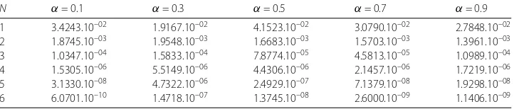
Table 2 The maximum error forN= 1,. . ., 6,λ1= 0.5,λ2= 0.5,β= 0.5 and different values of the parameterαin Example7.3

N α= 0.1 α= 0.3 α= 0.5 α= 0.7 α= 0.9

1 3.4243.10–02 _1.9167.10–02 _4.1523.10–02 _3.0790.10–02 _2.7848.10–02

2 1.8745.10–03 _1.9548.10–03 _1.6683.10–03 _1.5703.10–03 _1.3961.10–03

3 1.0347.10–04 _1.5833.10–04 _7.8774.10–05 _4.5813.10–05 _1.0989.10–04

4 1.5305.10–06 _5.5149.10–06 _4.4306.10–06 _2.1457.10–06 _1.7219.10–06

5 3.1330.10–08 _4.7322.10–06 _2.4929.10–07 _7.1379.10–08 _1.9298.10–08

6 6.0701.10–10 _1.4718.10–07 _1.3745.10–08 _2.6000.10–09 _1.1406.10–09

nandm. Form=n= 1 the approximate solution is exact and the truncated error is ob-served only. Form=n= 2 the approximate solution is exact whenN≥2. This pattern is observed for other parameters ofnandm, and the method gives the exact solution when-everN≥max{n,m}. Finally, we choosem=n= 12 to find the well-known exponential rate of convergence for Chebyshev spectral methods.

Example7.3 Consider the class of FPDEs of the form

∂αu(x,y)

∂xα –

∂βu(x,y)

∂yβ +u(x,y)

=λ1x1–αE1,2–α(λ1x)eλ2y

–λ2y1–βE1,2–β(λ2y)eλ1x+eλ1x+λ2y, (46)

subjected to the initial conditions

h(x) =eλ1x_{, g(y) =e}λ2y_{, h} 0= 1,

with free parameters λ1,λ2, α andβ. Here, En,m(Z) is the two-parameter function of

Mittag-Leffler type [52,53]. The exact solution iseλ1x+λ2y_{. In Table2, the maximum} er-rorE(N) is reported forN= 1, . . . , 6,λ1= 0.5,λ2= 0.5β= 0.5 andα= 0.1, 0.3, 0.5, 0.7, 0.9.

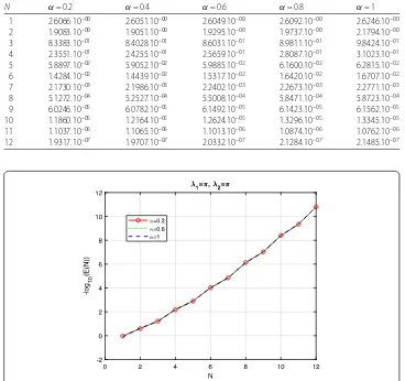
It shows the exponential rate of convergence for all values of theα. To illustrate this point we plotted the logarithm of maximum error in Fig.1. Table3shows the maximum error E(N) for negative parametersλ1= –0.5,λ2= –0.5.

Example7.4 Let us consider a class of FPDEs of the form

∂αu(x,y)

∂xα +ν

∂u(x,y)

∂y +u(x,y)

= –λ2₁x2–αE2,3–α

Figure 1The logarithm of maximum error versusN, for Example7.3

Table 3 The maximum error forN= 1,. . ., 6,λ1= –0.5,λ2= –0.5,β= 0.5 and different values of the parameterαin Example7.3

N α= 0.1 α= 0.3 α= 0.5 α= 0.7 α= 0.9

1 6.6793.10–03 _1.4736.10–02 _9.1582.10–03 _7.1919.10–03 _8.6468.10–03

2 4.3318.10–04 4.1717.10–04 3.5892.10–04 3.4776.10–04 3.3983.10–04 3 9.5043.10–05 4.8460.10–05 1.8542.10–05 1.2425.10–05 3.3041.10–05 4 3.5230.10–07 2.6035.10–06 1.4957.10–06 5.1700.10–07 3.8963.10–07 5 7.3145.10–09 2.6550.10–06 1.1231.10–07 2.2479.10–08 8.6745.10–09 6 1.3762.10–10 _7.8062.10–08 _6.9305.10–09 _1.0628.10–09 _3.6135.10–10

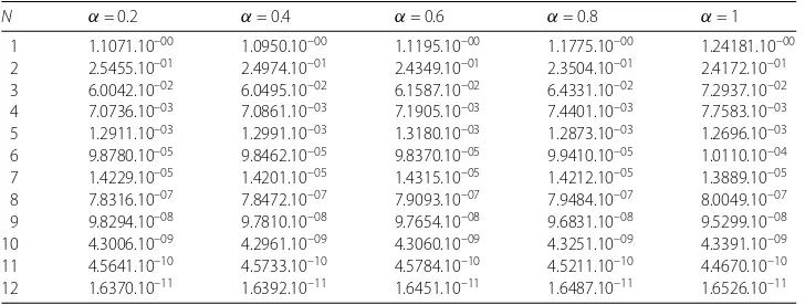
Table 4 The maximum error forN= 1,. . ., 12,λ1=π,λ2=π, and different values of the parameter αin Example7.4

N α= 0.2 α= 0.4 α= 0.6 α= 0.8 α= 1

1 1.1071.10–00 _1.0950.10–00 _1.1195.10–00 _1.1775.10–00 _1.24181.10–00

2 2.5455.10–01 _2.4974.10–01 _2.4349.10–01 _2.3504.10–01 _2.4172.10–01

3 6.0042.10–02 _6.0495.10–02 _6.1587.10–02 _6.4331.10–02 _7.2937.10–02

4 7.0736.10–03 _7.0861.10–03 _7.1905.10–03 _7.4401.10–03 _7.7583.10–03

5 1.2911.10–03 _1.2991.10–03 _1.3180.10–03 _1.2873.10–03 _1.2696.10–03

6 9.8780.10–05 _9.8462.10–05 _9.8370.10–05 _9.9410.10–05 _1.0110.10–04

7 1.4229.10–05 _1.4201.10–05 _1.4315.10–05 _1.4212.10–05 _1.3889.10–05

8 7.8316.10–07 _7.8472.10–07 _7.9093.10–07 _7.9484.10–07 _8.0049.10–07

9 9.8294.10–08 _9.7810.10–08 _9.7654.10–08 _9.6831.10–08 _9.5299.10–08

10 4.3006.10–09 _4.2961.10–09 _4.3060.10–09 _4.3251.10–09 _4.3391.10–09

11 4.5641.10–10 _4.5733.10–10 _4.5784.10–10 _4.5211.10–10 _4.4670.10–10

12 1.6370.10–11 _1.6392.10–11 _1.6451.10–11 _1.6487.10–11 _1.6526.10–11

+cos(λ1x)

λ2cos(λ2y) +sin(λ2y)

(47)

subjected to the initial conditions

h(x) = 0, g(y) =sin(λ2y), h0= 0,

Table 5 The maximum error forN= 1,. . ., 12,λ1= 2π,λ2= 2π, and different values of the parameterαin Example7.4

N α= 0.2 α= 0.4 α= 0.6 α= 0.8 α= 1

1 2.6066.10–00 _2.6051.10–00 _2.6049.10–00 _2.6092.10–00 _2.6246.10–00

2 1.9083.10–00 _1.9051.10–00 _1.9295.10–00 _1.9737.10–00 _2.1794.10–00

3 8.3383.10–01 _8.4028.10–01 _8.6031.10–01 _8.9811.10–01 _9.8424.10–01

4 2.3551.10–01 _2.4255.10–01 _2.5659.10–01 _2.8087.10–01 _3.1023.10–01

5 5.8897.10–02 _5.9052.10–02 _5.9885.10–02 _6.1600.10–02 _6.2815.10–02

6 1.4284.10–02 _1.4439.10–02 _1.5317.10–02 _1.6420.10–02 _1.6707.10–02

7 2.1730.10–03 _2.1986.10–03 _2.2402.10–03 _2.2673.10–03 _2.2771.10–03

8 5.1272.10–04 _5.2527.10–04 _5.5008.10–04 _5.8471.10–04 _5.8723.10–04

9 6.0246.10–05 _6.0782.10–05 _6.1492.10–05 _6.1423.10–05 _6.1562.10–05

10 1.1860.10–05 1.2164.10–05 1.2624.10–05 1.3296.10–05 1.3345.10–05 11 1.1037.10–06 1.1065.10–06 1.1013.10–06 1.0874.10–06 1.0762.10–06 12 1.9317.10–07 1.9707.10–07 2.0332.10–07 2.1284.10–07 2.1485.10–07

Figure 2The logarithm of maximum error versusN, forλ1=λ2=π, in Example7.4

π, and Table5shows these values forλ1=λ2= 2π. Though these tables show that

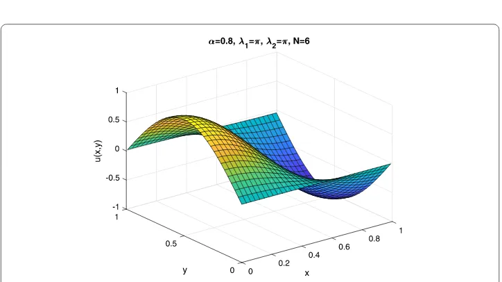
increas-ing the frequencyf =₂λ_π increase the absolute maximum error, the logarithm of maximum error plotted in Figs.2and3shows that both experiments of this example are of exponen-tial rate. To show the effectiveness of the method we also illustrated a numerical solution in Figs.4and5.

8 Applications

Example8.1 The advection is the transport of a substance by bulk motion. The model has been obtained by many restrictions such as neglecting friction and other parameters which dissipate energy. The dynamics of this phenomenon is described by

∂u(x,t)

∂t +ν

∂u(x,t)

∂x =f(x,t), (48)

Figure 3The logarithm of maximum error versusN, forλ1=λ2= 2π, in Example7.4

Figure 4The approximate solution forλ1=λ2=π, in Example7.4

to add a term containing a fractional derivative for dissipating energy in the advection equations and we have

∂u(x,t)

∂t +ν

∂u(x,t)

∂x +η

∂α_u(x,t)

∂xα =f(x,t), (49)

whereηis a constant and 0 <α≤1.

Now we consider a source function of the form f(x,t) =sin(λx+ωt), withλ=π and

Figure 5The approximate solution forλ1=λ2= 2π, in Example7.4

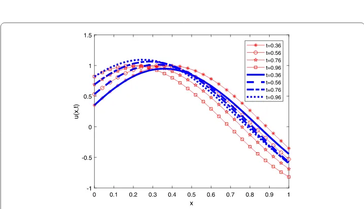
Figure 6Approximate solutions of the advection equation: the red line shows the approximate solutions without fractional term and the blue line shows the approximate solutions with a fractional term

fractional term decreases. This reduction in the density of particles can be explained by considering the dissipating of energy by friction and other physical parameters which we included by adding fractional terms.

Example8.2 Lighthill–Whitham–Richards (LWR) equation. The equation

∂β_u(x,y)

∂xβ +λ

∂β_u(x,y)

∂yβ = 0 (50)

has been extensively studied for describing a vehicular traffic flow on a finite-length high-way by using local fractional directive [1]. Here, the parametersλand 0 <β≤1 are known real numbers. Let us consider an example of this model with parametersλ= 1 andβ= 0.5 subjected to the initial conditionsh(x) =sinhβ(xβ_{),g(y) = –sinhβ(y}β_{) andh}

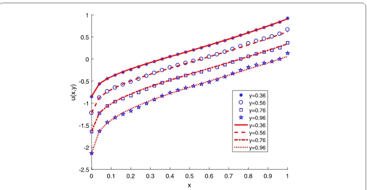
Figure 7The scaled solution of Lighthill–Whitham–Richards equation with Caputo-fractional derivatives (markers with blue color) and local fractional derivatives (lines with red color) withβ= 0.5 andλ= 1

that

sinhβ(x) := x

Γ(β+ 1)+ x3

Γ(3β+ 1)+· · ·

and

coshβ(x) := 1 + x

2

Γ(2β+ 1)+ x4

Γ(4β+ 1)+· · ·

are fractional generalizations of hyperbolic functions.

Kumar et al. [1] have obtained the general solution of Eq. (50) with local fractional derivatives as follows:

u(x,y) =sinhβ

xβcoshβ

xβ–coshβ

xβsinhβ

xβ. (51)

Now, we solve this equation with fractional derivatives in the Caputo sense by our pro-posed method. We observe that this solution shows a similar behavior to the solution obtained in (51) despite the differences in their definitions of fractional derivatives. In Fig.7, the scaled solutions of Eq. (50) with Caputo-fractional derivatives and local frac-tional derivatives are depicted. This comparison shows that we can also use the Caputo-fractional derivatives for describing a vehicular traffic flow in the Lighthill–Whitham– Richards model.

9 Conclusion

obtained by solving an algebraic equation. The numerical examples show that the intro-duced method gives the exact solution whenever the solution is a polynomial and the approximate solution converges very rapidly with an exponential rate for other examples. A generalization of our introduced method for nonlinear equations is more challenging than the linear case. Parallel to this work, it seems that the finite-difference methods also can efficiently be generalized and studied for linear and nonlinear equations. Therefore, we consider these topics for future studies and investigations.

Funding Not applicable.

Availability of data and materials Not applicable.

Competing interests

The authors declare that they have no competing interests.

Authors’ contributions

All the authors drafted the manuscript, and read and approved the final manuscript.

Publisher’s Note

Springer Nature remains neutral with regard to jurisdictional claims in published maps and institutional affiliations.

Received: 28 May 2019 Accepted: 22 October 2019 References

1. Kumar, D., Tchier, F., Singh, J., Baleanu, D.: An efficient computational technique for fractal vehicular traffic flow. Entropy20, 259 (2018)

2. Kumar, D., Singh, J., Baleanu, D., Rathore, S.: Analysis of a fractional model of the Ambartsumian equation. Eur. Phys. J. Plus133, 259 (2018)

3. Podlubny, I.: Fractional Differential Equations: An Introduction to Fractional Derivatives, Fractional Differential Equations, to Methods of Their Solution and Some of Their Applications, vol. 198. Academic Press, San Diego (1998) 4. Kilbas, A.A.A., Srivastava, H.M., Trujillo, J.J.: Theory and Applications of Fractional Differential Equations, vol. 204.

Elsevier Science Limited, Amsterdam (2006)

5. Kumar, D., Singh, J., Purohit, S.D., Swroop, R.: A hybrid analytical algorithm for nonlinear fractional wave-like equations. Math. Model. Nat. Phenom.14, 304 (2019)

6. Baleanu, D.: Fractional Calculus: Models and Numerical Methods, vol. 3. World Scientific, Singapore (2012) 7. Shiri, B., Baleanu, D.: System of fractional differential algebraic equations with applications. Chaos Solitons Fractals

120, 203–212 (2019)

8. Kumar, D., Singh, J., Tanwar, K., Baleanu, D.: A new fractional exothermic reactions model having constant heat source in porous media with power, exponential and Mittag-Leffler laws. Int. J. Heat Mass Transf.138, 1222–1227 (2019) 9. Kumar, D., Singh, J., Baleanu, D.: A new fractional model for convective straight fins with temperature-dependent

thermal conductivity. Therm. Sci.1, 1–12 (2017)

10. Singh, J., Kumar, D., Baleanu, D.: New aspects of fractional Biswas–Milovic model with Mittag-Leffler law. Math. Model. Nat. Phenom.14, 303 (2019)

11. Sedgar, E., Celik, E., Shiri, B.: Numerical solution of fractional differential equation in a model of HIV infection of CD44 (+) T cells. Int. J. Appl. Math. Stat.56, 23–32 (2017)

12. Mohammadi, F., Moradi, L., Baleanu, D., Jajarmi, A.: A hybrid functions numerical scheme for fractional optimal control problems: application to nonanalytic dynamic systems. J. Vib. Control24, 5030–5043 (2018)

13. Baleanu, D., Jajarmi, A., Asad, J.: The fractional model of spring pendulum: new features within different kernels. Proc. Rom. Acad., Ser. A19, 447–454 (2018)

14. Baleanu, D., Sajjadi, S.S., Jajarmi, A., Asad, J.H.: New features of the fractional Euler–Lagrange equations for a physical system within non-singular derivative operator. Eur. Phys. J. Plus134, 181 (2019)

15. Hajipour, M., Jajarmi, A., Baleanu, D., Sun, H.: On an accurate discretization of a variable-order fractional reaction-diffusion equation. Commun. Nonlinear Sci. Numer. Simul.69, 119–133 (2019)

16. Odibat, Z., Momani, S.: The variational iteration method: an efficient scheme for handling fractional partial differential equations in fluid mechanics. Comput. Math. Appl.58, 2199–2208 (2009)

17. Jafari, H., Nazari, M., Baleanu, D., Khalique, C.M.: A new approach for solving a system of fractional partial differential equations. Comput. Math. Appl.66, 838–843 (2013)

18. Gupta, A., Ray, S.S.: Numerical treatment for the solution of fractional fifth-order Sawada–Kotera equation using second kind Chebyshev wavelet method. Appl. Math. Model.39, 5121–5130 (2015)

19. Gupta, A., Ray, S.S.: The comparison of two reliable methods for accurate solution of time-fractional Kaup–Kupershmidt equation arising in capillary gravity waves. Math. Methods Appl. Sci.39, 583–592 (2016) 20. Ray, S.S., Gupta, A.: Numerical solution of fractional partial differential equation of parabolic type with Dirichlet

21. Wu, J.-L.: A wavelet operational method for solving fractional partial differential equations numerically. Appl. Math. Comput.214, 31–40 (2009)

22. Wang, L., Ma, Y., Meng, Z.: Haar wavelet method for solving fractional partial differential equations numerically. Appl. Math. Comput.227, 66–76 (2014)

23. Jafari, H., Daftardar-Gejji, V.: Solving linear and nonlinear fractional diffusion and wave equations by Adomian decomposition. Appl. Math. Comput.180, 488–497 (2006)

24. Jafari, H., Seifi, S.: Solving a system of nonlinear fractional partial differential equations using homotopy analysis method. Commun. Nonlinear Sci. Numer. Simul.14, 1962–1969 (2009)

25. Chen, Y., Sun, Y., Liu, L.: Numerical solution of fractional partial differential equations with variable coefficients using generalized fractional-order Legendre functions. Appl. Math. Comput.244, 847–858 (2014)

26. Baseri, A., Babolian, E., Abbasbandy, S.: Normalized Bernstein polynomials in solving space-time fractional diffusion equation. Adv. Differ. Equ.1, 346 (2017)

27. Baleanu, D., Shiri, B.: Collocation methods for fractional differential equations involving non-singular kernel. Chaos Solitons Fractals116, 136–145 (2018)

28. Hajipour, M., Jajarmi, A., Baleanu, D.: On the accurate discretization of a highly nonlinear boundary value problem. Numer. Algorithms79, 679–695 (2018)

29. Hajipour, M., Jajarmi, A., Malek, A., Baleanu, D.: Positivity-preserving sixth-order implicit finite difference weighted essentially non-oscillatory scheme for the nonlinear heat equation. Appl. Math. Comput.325, 146–158 (2018) 30. Baleanu, D., Shiri, B., Srivastava, H., Al Qurashi, M.: A Chebyshev spectral method based on operational matrix for

fractional differential equations involving non-singular Mittag-Leffler kernel. Adv. Differ. Equ.1, 353 (2018) 31. Bhrawy, A.H., Zaky, M.A., Machado, J.A.T.: Numerical solution of the two-sided space-time fractional telegraph

equation via Chebyshev tau approximation. J. Optim. Theory Appl.174, 321–341 (2017)

32. Dabiri, A., Butcher, E.A.: Numerical solution of multi-order fractional differential equations with multiple delays via spectral collocation methods. Appl. Math. Model.56, 424–448 (2018)

33. Dabiri, A., Butcher, E.A.: Stable fractional Chebyshev differentiation matrix for the numerical solution of multi-order fractional differential equations. Nonlinear Dyn.90, 185–201 (2017)

34. Doha, E.H., Bhrawy, A.H., Baleanu, D., Ezz-Eldien, S.S.: The operational matrix formulation of the Jacobi tau approximation for space fractional diffusion equation. Adv. Differ. Equ.,2014, 231 (2014)

35. Doha, E.H., Bhrawy, A., Ezz-Eldien, S.S.: A Chebyshev spectral method based on operational matrix for initial and boundary value problems of fractional order. Comput. Math. Appl.62, 2364–2373 (2011)

36. Han, W., Chen, Y.-M., Liu, D.-Y., Li, X.-L., Boutat, D.: Numerical solution for a class of multi-order fractional differential equations with error correction and convergence analysis. Adv. Differ. Equ.2018, 253 (2018)

37. Kojabad, E.A., Rezapour, S.: Approximate solutions of a sum-type fractional integro-differential equation by using Chebyshev and Legendre polynomials. Adv. Differ. Equ.2017, 351 (2017)

38. Hou, J., Yang, C.: Numerical solution of fractional-order Riccati differential equation by differential quadrature method based on Chebyshev polynomials. Adv. Differ. Equ.2017, 365 (2017)

39. Khaleghi, M., Babolian, E., Abbasbandy, S.: Chebyshev reproducing kernel method: application to two-point boundary value problems. Adv. Differ. Equ.2017, 26 (2017)

40. Mason, J.C., Handscomb, D.C.: Chebyshev Polynomials. CRC Press, Boca Raton (2002)

41. Bhrawy, A., Zaxy, M., Baleanu, D., Abdelkawy, M.: A novel spectral approximation for the two-dimensional fractional sub-diffusion problems. Rom. J. Phys.60, 344–359 (2015)

42. Zaky, M.A., Doha, E.H., Taha, T.M., Baleanu, D.: New recursive approximations for variable-order fractional operators with applications. Math. Model. Anal.23, 227–239 (2018)

43. Bhrawy, A., Zaky, M.A.: Highly accurate numerical schemes for multi-dimensional space variable-order fractional Schrödinger equations. Comput. Math. Appl.73, 1100–1117 (2017)

44. Zaky, M.A.: Recovery of high order accuracy in Jacobi spectral collocation methods for fractional terminal value problems with non-smooth solutions. J. Comput. Appl. Math.357, 103–122 (2019)

45. Bhrawy, A., Zaky, M.: A fractional-order Jacobi tau method for a class of time-fractional PDEs with variable coefficients. Math. Methods Appl. Sci.39, 1765–1779 (2016)

46. Bhrawy, A., Zaky, M.A.: A method based on the Jacobi tau approximation for solving multi-term time-space fractional partial differential equations. J. Comput. Phys.281, 876–895 (2015)

47. Zaky, M.A.: AA Legendre spectral quadrature tau method for the multi-term time-fractional diffusion equations. Comput. Appl. Math.37, 3525–3538 (2018)

48. Zaky, M.A.: An improved tau method for the multi-dimensional fractional Rayleigh–Stokes problem for a heated generalized second grade fluid. Comput. Math. Appl.75, 2243–2258 (2018)

49. Bhrawy, A., Zaky, M.A., Van Gorder, R.A.: A space-time Legendre spectral tau method for the two-sided space-time Caputo fractional diffusion-wave equation. Numer. Algorithms71, 151–180 (2016)

50. Trefethen, L.N.: Is Gauss quadrature better than Clenshaw–Curtis? SIAM Rev.50, 67–87 (2008) 51. Chawla, M.: Error estimates for the Clenshaw–Curtis quadrature. Math. Comput.22, 651–656 (1968) 52. Srivastava, H.M.: Some families of Mittag-Leffler type functions and associated operators of fractional calculus

(survey). TWMS J. Pure Appl. Math.7, 123–145 (2016)

53. Tomovski, Ž., Hilfer, R., Srivastava, H.M.: Fractional and operational calculus with generalized fractional derivative operators and Mittag-Leffler type functions. Integral Transforms Spec. Funct.21, 797–814 (2010)

54. El-Sayed, A., Behiry, S., Raslan, W.: Adomian’s decomposition method for solving an intermediate fractional advection–dispersion equation. Comput. Math. Appl.59, 1759–1765 (2010)