A new approach to the hourly mean computation problem
when dealing with missing data
S. Marsal and J. J. Curto
Observatori de l’Ebre. CSIC — Universitat Ramon Llull Carretera de l’Observatori, 8. 43520 Roquetes, Spain
(Received November 7, 2008; Revised May 8, 2009; Accepted May 14, 2009; Online published October 19, 2009)
Geomagnetic observatory records are unavoidably affected by primary data interruptions which, in turn, may have possible effects on the accuracy of the definitive data derived from them. One of the products most widely used by the scientific community is the mean hourly values, immediately obtained from the primary minute values of the geomagnetic field. Although some precepts have already been proposed and used, a definitive criterion regarding the procedure to follow when dealing with missing data has not yet been established. This could be seen in the last IAGA meetings and workshops, where several constructive opinions were put forward in this respect. The present discussion is devoted to analyzing the effects that different amounts of missing data have upon the accuracy of the means, a necessary step before establishing a definitive rule as to how to deal with these situations. In this statistical approach, we propose a new criterion based on the relative value of the root mean square error (between actual and computed means) with respect to the natural magnetic field variations of the original hourly interval.
Key words: Mean hourly values, uncertainty, geomagnetism, accuracy, confidence level, missing data, data processing, statistics.
1.
Introduction
The mean hourly values of the Earth’s magnetic field el-ements as recorded by ground-based observatories are used in a number of studies dealing with medium term
varia-tions, such as those related to the Sq system of currents
(Green, 1972; Tortaet al., 1997) or the EEJ (Rangarajan,
1982). They are also employed in magnetic field modelling
(Walkeret al., 1997), indexing (Martini and Mursula, 2006;
Svalgaard and Cliver, 2007), and even in the study of Sq
trends (Le Mou¨el et al., 2005; Torta et al., 2008). They
provide representative values of the magnetic field within the hours of interest, which are useful when dealing with intermediate timescale magnetic features. Regarding the cases of long and short timescales, high time resolutions are required when studying shorter timescale magnetic phe-nomena such as Pi2 (1-second data) or Sfe (1-minute data), while low time resolutions are used in the study of longer timescale phenomena such as magnetic jerks (monthly val-ues) or secular variation (annual valval-ues).
A moderate time resolution also implies that high accu-racy in the magnetic field magnitude is simply not required for many purposes. Hence we are faced with the question as to what the required level of accuracy for the hourly means is. For practical reasons the answer to this question should be as general as possible, although it probably depends on several factors, such as the type of study carried out by each particular data user. Likewise, it seems clear that the degree of magnetic field disturbance in the relevant hourly
inter-Copyright cThe Society of Geomagnetism and Earth, Planetary and Space Sci-ences (SGEPSS); The Seismological Society of Japan; The Volcanological Society of Japan; The Geodetic Society of Japan; The Japanese Society for Planetary Sci-ences; TERRAPUB.
val also plays an important role. Suppose, for instance, that the magnetic field variation during a given disturbed hourly interval is 500 nT. For many purposes it will probably be meaningless to provide a mean hourly value (MHV) with an accuracy of 1 nT, since it will not add substantial infor-mation to our study. An accuracy of 50 nT may well suffice. On the contrary, an hourly variation of 5 nT will certainly require a more accurate mean to distinguish the fine natu-ral variations we may be interested in, such as those related
to the Sq. Following this reasoning, we hereafter suggest
establishing a criterion based on the standard deviation of the magnetic field variations computed from the (original) minute values in the hour, rather than establishing one def-inite, clear-cut value for accuracy. Thus, the question to be addressed to MHV data users is: What fraction of the standard deviation represents the required MHV accuracy? The answer to this question requires a deep analysis of the diverse uses of MHVs that we, as data providers, will not attempt to undertake here.
The problem of missing data within the hourly intervals is related to this issue. An absence of data is frequently a consequence of acquisition problems, or is derived from the data post-processing itself. There are several opinions regarding the most adequate procedure to follow in the pres-ence of data gaps, as shown in the last IAGA meetings and workshops. One of the fundamental questions to be addressed is: How many minute data can be lost in one hour without the hourly mean losing significance? This is directly related to the question addressed in the previous paragraph regarding the required accuracy of the MHVs. If the reported mean stays within the required accuracy de-spite a given number of missing data, then this number is
Table 1. Geomagnetic and geographic coordinates of the observatories used in this study.
Geomagnetic latitude Geomagnetic longitude Geographic latitude Geographic longitude
(◦N) (◦E) (◦N) (◦E)
College, CMO 65.4 261.7 64.9 212.2
Boulder, BOU 48.4 320.6 40.1 254.8
San Juan, SJG 28.3 6.1 18.1 293.8
Ebre, EBR 43.2 81.3 40.8 0.5
Livingston Is., LIV −52.6 8.6 −62.7 299.6
considered permissible. Of course, this question cannot be
answereda posteriori, since we would not be able to
cal-culate theactualortruemean (i.e., with the complete data
set). In this sense, the aim of the exhaustive works of Man-dea (2002) and Schott and Linthe (2007) was to establish a
rule capable of,a priori, answering the following question:
Given a tolerable number of missing data, to what extent
does theestimatedmean depart from theactualmean? In
their studies, these authors find major dependences on the latitude of the analyzed observatory and on the underlying magnetic field activity, which leave questions unanswered regarding the MHV computation problem.
Our approach differs slightly in that, given a number of missing data, we are interested in finding out by what
frac-tion of the standard deviafrac-tion (of the original data) the
es-timatedmean departs from theactualmean. For now, let
us refer to this concept asrelative accuracy. For the same
reasons as those set out above, we think this is a more phys-ically significant parameter than an absolute lower limit for the accuracy (e.g., 1 nT). Obviously, there are so many possibilities of different distributions of gaps within the hour, and the level of magnetic activity of the lost data, that the outcome will be a distribution of probability. If the aforementioned required relative accuracy were well-established, the question of missing data could be addressed in the following way: What is the maximum number of missing data we can permit, while being reasonably
confi-dent that the (pre-established) requiredrelativeaccuracy is
still achieved? We will situate this confidence level at 95% probability; in other words, we will say we are reasonably confident that the required limit of relative accuracy will not be surpassed if its probability of occurrence is less than 5%. Because it is useful for error propagation, we are also
in-terested here in therelativestandard deviation between the
estimated and actual means.
Given that we will not assume any pre-established rela-tive level of accuracy for the MHVs, in the following sec-tions we will invert the previous question and try to provide an answer to the equivalent one: What is the relative ac-curacy of the estimated MHV when dealing with different numbers of missing data, whether they be 2, 10, 35, 50...? Once the required relative accuracy has been determined (by others), the answer to the last question will immediately allow us to set the maximum number of missing data.
2.
Procedure and Results
The answer to the last question demands a statistical anal-ysis based on real data. Given a complete test hour (i.e., with no missing data), how does the mean respond to the (artificial) extraction of minute values? As pointed out
be-fore, it will depend on the way these data are extracted. Among other interesting points, the work from Schott and Linthe (2007) performs a complete analysis on the real dis-tribution of data and gap segments within the hourly inter-vals of a given station (PAF). It concludes that the prob-ability of having more than one gap segment per hour is relatively small (of the order of 10% or less); likewise, our calculations for the Ebro Observatory for the period 2001– 2005 yield a 94% probability for a 1 gap segment and 6% for 2 gap segments, with cases of 3 or more segments be-ing virtually non-existent. In fact, Mandea (2002) takes as a working hypothesis a single gap segment of variable length. In this work we will proceed by following two scenarios: in the first one data are extracted randomly to simulate randomly scattered missing data, while in the second one data are extracted as a continuum to simulate one single gap. As a rule, and assuming a fixed number of missing data, the greater the number of gap segments within the hourly interval, the closer both the estimated and actual means are. We can see this intuitively as the information lost with a short gap segment can, to a certain extent, be interpolated by the neighbouring minutes. Hence, although the first case is generally unlikely, it will be useful to show how different the results from both situations are. Finally, an upper limit is established for the uncertainty of the estimated mean when
dealing with a realistic distribution of missing data, i.e.,
considering the adequate proportion of gap segments. The real data used in this study are taken from geo-magnetic stations at different latitudes: College (CMO) at high latitude, Boulder (BOU) at mid-latitude, and San Juan
(SJG) at low latitude, for which the X magnetic element
was analyzed. Furthermore, we have made use of the H
element of the observatories run by the authors, namely the Ebro (EBR) and Livingston Island (LIV) ones, see Table 1. The use of these magnetic elements is due to their greater impact in indexing and modelling practices. The data have also been selected in such a way that they cover different
magnetic activity levels: active, A (local K-index = 8),
moderate, M (K = 5) and quiet intervals, Q (K = 0).
24 hours have been used for a given observatory and
dis-turbance level, so that a total of 360 (5 stations×3 activity
levels×24 h) hourly intervals have been analyzed.
Our immediate objective is to obtain the uncertainty of
the mean computed when possessing 60−g data points,
whereg is the number of missing data. We will proceed
by following a Type A evaluation, as defined in the Guide to the Expression of Uncertainty in Measurement (‘GUM’, ISO, 1993), in accordance with the subsequent steps:
2
0 0 40 6
Minute number
0 11500
11600 11700 11800 11900 12000
X (nT
)
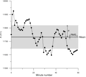
Mean RMS-5
Fig. 1. X-component minute values of the disturbed hourly interval recorded at the CMO observatory on January 17th, 2005, 09:00–10:00 UT. The standard deviationσand the RMS value obtained after random extraction of 5 data points are also displayed.
complete hourly interval for testing.
(2) g minute values are deleted from the selected hourly
interval and the new (or estimated) meanx−gis
com-puted
(3) The actual meanx0 (i.e., with no deletions) is
sub-tracted fromx−g.
(4) The preceding steps are repeated for different
extrac-tion combinaextrac-tions of g data points within the same
hourly interval. The values xi−g − x0 are thus
obtained, where the i index denotes each particular
choice of extraction.
(5) The root mean square of these differences is computed by means of Eq. (1):
RMS−g =
l
i=1
xi
−g− x0 2
l−1 (1)
(6) The 95th percentile of the distribution of the differ-ences obtained in step 4 is computed, giving rise to the so-called ‘uncertainty at the level of confidence of 95%’,U−95g(see ISO, 1993).
(7) The quotients RMS−g/σ and U−95g/σ are computed,
whereσ is the standard deviation of the geomagnetic
data in the original hourly interval and gives an idea of the natural magnetic field activity.
We can interpret RMS−g as a representative value of the
deviation of the new mean (after the extraction of g data
minutes) from the actual mean. Note that the RMS value
obtained from Eq. (1) is notstricto sensuthe standard
devi-ation of the distribution of the differences as, in general, the
mean of the differentxi
−g (with respect toi) is different
fromx0. Our aim is to study the statistical response of
ap-plying steps 1 to 7 (with differentgvalues) to the different
360 hourly intervals.
2.1 Random extraction
In this case, the data in our test hourly interval are
elimi-nated in a random way, so that for each numbergof
miss-ing data, 1000 different extraction combinations are made
(i.e.,l =1000 in Eq. (1)). For example, forg =5 a first
choice of deletions (l =1) might correspond to minutes 12,
18, 31, 44 and 57, forl =2 the deleted minutes might be
00, 07, 23, 24 and 44, and so on. A series of tests
indi-cate thatl=1000 provides a sample large enough to obtain
significant results. This will give rise to a distribution of the differences between estimated and actual means, which we will show to be well-approximated by a normal distri-bution centred at zero. This fact will permit us to note that
(only for the case of random extraction) the RMS/σ value
is effectively the same as therelativestandard deviation of
the distribution. After many observations we will arrive at the important result that, whatever the hourly interval we consider (regardless of the latitude or activity level), this
relativestandard deviation is constant for a given number of missing data. With these results, we will infer the 95%
confidence level to be the value given by twice the RMS/σ.
Finally, we will provide a plain statistical justification that approximates the results we find.
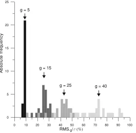
Figure 1 shows the minute values of the active (A) hourly interval corresponding to January 17th, 2005, 09:00– 10:00 UT as recorded at the CMO observatory. The differ-ences of the means after randomly extracting 5 data minutes are distributed as shown in Fig. 2. Note that Fig. 1 also
dis-playsσ, the standard deviation of the 60 minute values of
the geomagnetic field, and RMS−5obtained from the
distri-bution of Fig. 2.
en--12 -10 -8 -6 -4 -2 0 2 4 6 8 10 12 14 <x>-5 - <x>0 (nT)
0 40 80 120
A
bso
lut
e
fr
eq
u
e
n
c
y
Fit Results
Fit 1: Normal
Number of data points used = 1000 Average X = -0.0645515 Standard Deviation = 3.3797
Fig. 2. Histogram showing the distribution of the 1000 differences of the means obtained after random extraction of 5 data points for a high-latitude observatory (CMO) and high activity level (A); hourly interval: January 17th, 2005, 09:00–10:00 UT.
-0.06 -0.05 -0.04 -0.03 -0.02 -0.01 0 0.01 0.02 0.03 0.04 0.05 0.06
<x>-5 - <x>0 (nT)
0 100 200 300 400
Abso
lut
e
freq
u
e
nc
y
Fit Results
Fit 1: Normal
Number of data points used = 1000 Average X = 0.000133333 Standard Deviation = 0.018862
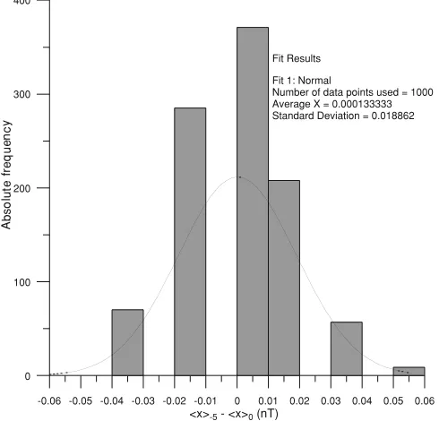
Fig. 3. Distribution of the 1000 means after random extraction of 5 data points for the hourly interval 00:00–01:00, Nov 16th, 2005, for SJG Q (quiet). Note that the Gaussian curve does not fit the observed data well. The striped structure of the distribution is an effect of the limited resolution of the primary minute data applied to such an extremely quiet interval.
countered for the hourly interval of our example when
ap-plying different values ofg. It is worth mentioning that the
RMS value as computed from Eq. (1) is 3.38 nT (Table 2), which coincides with the standard deviation of the distribu-tion of the estimated means (fit results in Fig. 2). This is not only the case for the hourly interval of Fig. 2 but, rather, it is a general result observed whenever dealing with ran-dom extraction, due to the fact that the distribution is well
centred atx0 (xi−5− x0 = −0.06 nT from Fig. 2).
The reader can find another example in Fig. 3. As stated
in the introduction of Section 2, this assertion is not valid in general, as we will see when dealing with the case of continuous extraction (Section 2.2).
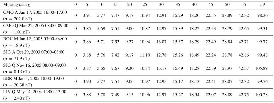
ad-Table 2. Root mean square (Eq. (1)) of the computed means aftergrandom deletions, and percentages with respect toσ. Application to the hourly interval of Fig. 2.
Missing datag 0 5 10 15 20 25 30 35 40 45 50 55 59
RMS−g(nT) 0 3.38 5.04 6.47 7.95 9.42 11.20 13.13 15.80 19.55 24.94 37.24 86.48
RMS−g/σ(%) 0 3.89 5.80 7.44 9.15 10.83 12.89 15.11 18.18 22.49 28.68 42.83 99.47
Table 3. Relative values of the root mean square (RMS−g/σ(%)) after extraction ofgdata points for a wide sample of stations and activity levels (A
active, M moderate, Q quiet). Note the relatively constant value in a given column, even for hours with differentσvalues.
Missing datag 0 5 10 15 20 25 30 35 40 45 50 55 59
CMO A Jan 17, 2005 16:00–17:00
0 3.91 5.77 7.47 9.17 10.94 12.91 15.29 18.20 22.55 28.89 42.32 98.36 (σ =702.0 nT)
CMO Q Mar 22, 2005 08:00–09:00
0 3.85 5.69 7.51 9.00 10.87 12.97 15.39 18.22 22.53 28.79 42.65 99.31 (σ =1.01 nT)
BOU M Jan 12, 2005 03:00–04:00
0 3.86 5.71 7.53 9.27 10.94 13.07 15.37 18.29 22.49 28.84 42.71 99.77 (σ =18.9 nT)
SJG A Oct 29, 2003 07:00–08:00
0 3.88 5.76 7.42 9.17 11.10 12.78 15.26 18.49 22.24 28.78 42.86 99.48 (σ =71.9 nT)
SJG Q Nov 16, 2005 08:00–09:00
0 3.87 5.65 7.67 9.30 10.84 13.17 15.49 18.28 22.39 28.97 42.37 105.89 (σ =0.13 nT)
EBR M Jan 1, 2005 18:00–19:00
0 3.90 5.77 7.51 9.06 10.97 12.95 15.17 18.13 22.41 28.87 42.32 99.76 (σ =20.38 nT)
LIV Q May 14, 2004 12:00–13:00
0 3.88 5.78 7.49 9.15 10.96 12.97 15.27 18.54 22.07 28.89 42.75 100.28 (σ =2.40 nT)
Table 4. Relative uncertainty at the level of confidence of 95%,U95
−g/σ, after random extraction ofgdata minutes. The values are roughly twice those
of Table 3.
Missing datag 0 5 10 15 20 25 30 35 40 45 50 55 59
U−95g/σ(%) 0 7.8 11.5 15 18 22 26 31 37 45 58 85 ≈200
justed by a Gaussian curve. This agreement has also been checked for many other hourly intervals; as expected, the least favourable cases are found with quiet intervals, when
gis either small or large (see Fig. 3). Nevertheless,
regard-ing the parameters we are interested in, a normal
(Gaus-sian) distribution is still suitable even in this case. A test
for this is the value ofU95
−gas the observed 95th percentile
of the distribution: should the data benormallydistributed,
the 95th percentile (=0.0379 nT in the case of Fig. 3,
ob-tained after the elimination of the tail-most 5% of the
dis-tribution) must coincide with twice the value of the RMS−g
parameter (2·RMS−5 = 0.0377 nT, where RMS−5 is the
standard deviation displayed in the fit results of Fig. 3). In
summary, we infer that thenormaldistribution is adequate
to quantify our problem, and thus (only for the case of
ran-dom extraction), we will work with the hypothesis thatthe
resultant means following random extraction are normally distributed around the actual mean, regardless of the num-ber of missing data or activity level.
If we continue analyzing Table 2 we realize that, as
ex-pected, the root mean square increases withg, the number
of missing data. As stated, our approach consists in
normal-izing the RMS−g values with respect to the standard
devi-ationσ of the original data (with no deletions). If we do
so and multiply by 100 to obtain the percentages, we obtain the last row of Table 2.
A similar table has been obtained for each of the 360 an-alyzed hours to cover a wide spectrum of activity levels and
observatory latitudes. After this, we observed thatalthough
the different RMS−g vary, the percentages RMS−g/σσσσσσσσ
are practically the same, even if we put different sta-tions and activity levels together. Table 3 illustrates this important result with an assorted representation of latitudes and magnetic activities.
Let us refer to RMS−g/σ as the ‘relativestandard
uncer-tainty’ of the estimated mean after the extraction ofgdata
points. However, it should be clarified thatrelativein this
context means with respect toσ.
Assuming a normal distribution of the means (obtained after random extraction) around the actual mean, the
prob-ability that a given mean is within 2·RMS−g/σ is 95%,
which establishes our confidence level, so the values in
Ta-ble 3 must be duplicated to obtain U95/σ, which will be
referred to as the ‘relativeuncertainty at the level of
confi-dence of 95%’. In other words, after the random extraction of 5 data minutes, we can say it is reasonably unlikely that
the error in the newly computed mean surpasses 2×3.9%
=7.8% (see columng=5 in Table 3) of the standard
devi-ationσof the original hourly data. In conclusion, if we had
pre-established the requiredrelativeaccuracy, the
penulti-mate question in the introduction, regarding the maximum number of missing data acceptable, would then immedi-ately be answered with the help of Table 4, which is valid for any latitude and activity level.
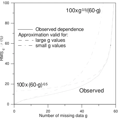
0 20 40 60 Number of missing data g
0
Fig. 4. Observed relative standard deviation after random extraction ofg
data points, together with approximations for large and smallgvalues.
values of the RMS−g/σparameter (Taylor, 1982). Suppose
that instead of being continuous, the magnetic field values
were distributed around the actual meanx0 according to
a random distribution with standard deviationσ (the actual
standard deviation of the original data). After the random elimination of 59 points from our original hourly interval, the mean deviation of the remaining 1 point with respect to
the true mean is just the standard deviationσ of the
sam-ple, so RMS−59/σ = 1 (i.e., 100%), which roughly
coin-cides with the results displayed in the last column of Ta-ble 3. Likewise, we know from fundamental statistics that after the elimination of 55 data points, the standard uncer-tainty of the mean obtained with the remaining 5 data points
is σ/√5, so RMS−55/σ = 1/
√
5 (i.e., 44.7%), which is
similar to the corresponding column with headerg = 55
in Table 3. In general, in possession ofn data points, the
mean relative deviation with respect to the actual mean is
RMS−g/σ = 1/
√
n = 1/√(60−g). Of course, in the
real case we are limited ton =60, where both actual and
estimated means must converge, so it is expectable that the deviation with respect to the true mean decreases faster than
1/√n. At the opposite extreme (small value ofg), after the
deletion of g data points, the best estimate of the sum of
the extracted data isgx0, with a standard uncertainty of
σ√g. This must coincide with the uncertainty of the sum
of the available data, where the best estimate for this sum is
(60−g)x0. The new mean equals the sum of the available
data divided by the number of available data, 60−g.
Con-sequently, the standard uncertainty of the new mean will be
(σ√g)/(60−g), or RMS−g/σ = √g/(60−g). Both
ap-proximations for small and largegvalues are displayed in
Fig. 4, together with the observed results.
2.2 Continuous extraction
Things are not so simple when considering the most com-mon case—that of one single gap. The procedure we follow in this case is exactly the same as with the previous one, but
instead of random extractions, we will consider a continu-ous extraction of variable length. The number of possible
ways a single gap of lengthgcan be extracted from a given
hour is reduced toc = 61−g, which allows an analysis
based on all the possible cases. Firstly, we will see that the approximation consisting in identifying RMS (Eq. (1)) with the standard deviation of the differences between esti-mated and actual means is, in general, no longer valid for the case of one single gap. Secondly, we will investigate
the behaviour of the RMS/σandU95/σparameters and see
that, unlike the previous case, they are not constant over dif-ferent hourly intervals. This will hinder our objectives, and force us to adopt uncertainty intervals for the corresponding
relative uncertainties themselves (i.e., RMS/σ andU95/σ).
However, we will not find a significant dependence of these two parameters on the observatory latitude or magnetic ac-tivity level, and this will allow us to set (universally) com-mon bounds for these intervals.
Figure 5 shows the distribution of the 41 differences of the estimated means with respect to the actual (or true) mean for the case of LIV M, hourly interval: January 9th, 2004, 18:00–19:00 UT, after extracting 20 running minutes
(c=61−20=41).
It is clear that the histogram of Fig. 5 is far from a normal distribution. Moreover, the mean computed after extracting 20 data minutes does not coincide, on average, with the
ac-tual meanx0. This is due to the distribution of the
mag-netic field values along the hourly interval, and to the fact that, with a continuous gap, the central minutes are more likely to be extracted than those at both ends of the inter-val. This also implies that the RMS value evaluated from Eq. (1) (3.5 nT in our example) is slightly different from the standard deviation of the distribution of the differences
xi
−20− x0 (3.1 nT), especially when dealing with long
gaps. Despite this, in the interests of readability we will
continue to refer to RMS−g/σ as the relative standard
un-certainty.
We are now interested in the distribution of the relative
standard uncertainties RMS−g/σ over different hourly
in-tervals. Given a gap lengthg, is the RMS−g/σ value
con-stant regardless of the magnetic activity and observatory considered, as it was for the random case considered in the previous section? If it were, we would be able to construct a table similar to Table 3 and provide the typical accuracy
of the mean estimated in the absence ofg continuous data
points. Figure 6 shows the distribution of the 24 RMS−g/σ
values corresponding to LIV M (moderate activity) for gap
lengthsg=5, 15, 25 and 40.
The same experiment of Fig. 6 for the case of random
extraction (Section 2.1) would have shownδ-like
distribu-tions. Thus, for example, all the 24 points corresponding to
g = 5 would be clustered around 3.9%, those forg = 15
around 7.5%, and so on (see Table 3). Unfortunately, this is not the case for the continuous extraction, so instead of a
spot value, the data are now distributed in a finiteinterval;
alternatively, we can understand this interval as reflecting the uncertainty of the parameter we are trying to evaluate,
RMS−g/σ, which in turn is also an uncertainty. In our
ex-ample, for a gap length g = 15, RMS−g/σ (%) =25%
-6 -5 -4 -3 -2 -1 0 1 2 3 4 5 6
<x>-20-<x>0 (nT)
0 4 8 12
A
bso
lut
e
fr
eq
ue
n
c
y
Mean of the distribution
Fig. 5. Histogram showing the distribution of the 41 possible differences of the means after extraction of 20-minute-long gaps from the hourly interval 18:00–19:00 UT, January 9th, 2004, station LIV.
0 10 20 30 40 50 60 70 80 90 100
RMS-g/ (%) 0
5 10 15 20 25
Ab
s
o
lu
te
fr
e
q
u
e
n
c
y
g = 5
g = 15
g = 25 g = 40
Fig. 6. Distribution of the individual RMS−g/σvalues (g=5, 15, 25 and 40) for the 24 hourly intervals of LIV M (moderate magnetic activity). For a
gap lengthg=15, for example, most of the 24 estimated means are between 20 and 30% ofσaway from the actual mean.
of the distribution associated to the relative standard uncer-tainty itself).
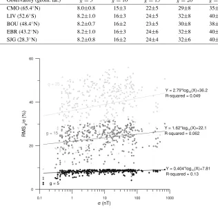
So far we have dealt with the particular case of LIV M, a mid-latitude observatory (as regards magnetic coordinates), but does the abovementioned interval increase with increas-ing latitude or activity level? Table 5 shows a poor or null
dependence of the RMS−g/σ interval on the observatory
latitude.
In addition to this, Fig. 7 aims to show the dependence
of the RMS−g/σ values on the degree of magnetic activity,
quantified here with the standard deviationσof the original
hourly data.
The plots on Fig. 7 deserve special attention. The most apparent features are:
- The data distribution suggests a linear relationship
be-tween the relative standard uncertainty RMS−g/σand
Table 5. Dependence of the RMS−g/σ(%) interval on the observatory latitude. Observatories are arranged in order from higher to lower geomagnetic
latitudes. For the computation of the RMS−g/σintervals in a given observatory, the three magnetic activity levels (A, M and Q) have been taken
together.
Observatory (geom. lat.) g=5 g=10 g=15 g=20 g=25
CMO (65.4◦N) 8.0±0.8 15±3 22±5 29±8 35±10
LIV (52.6◦S) 8.2±1.0 16±3 24±5 32±8 40±10
BOU (48.4◦N) 8.2±0.7 16±2 23±5 30±8 38±10
EBR (43.2◦N) 8.2±1.0 16±3 24±6 32±8 40±11
SJG (28.3◦N) 8.2±0.8 16±2 24±4 32±6 40± 8
0.1 1 10 100 1000
(nT)
0 20 40 60
RMS
-g
/(
%
)
Y = 0.404*log10(X)+7.81
R-squared = 0.13 Y = 1.62*log10(X)+22.1
R-squared = 0.062 Y = 2.79*log10(X)+36.2
R-squared = 0.049
g = 25
g = 15
g = 5
Fig. 7. Relative standard uncertainty, RMS−g/σ, as a function ofσfor the 360 hourly intervals after extraction of gap segments of lengthg=5, 15
and 25.
data, log10(σ), with the slope increasing with the gap
length.
- Simultaneously, the noticeable scatter enhancement
experienced for increasing gap lengths,g, greatly
over-shadows theσ dependencies, resulting in small
corre-lation coefficients (R-squared in the figure).
- For a given gap lengthg, the scatter is slightly reduced
with increasingσ.
- For a given gap length, the data are not symmetrically distributed around the mean, and the tail of the
distri-bution is elongated towards low values of RMS−g/σ.
On the contrary, an accumulation of data points is ob-served in the upper part of the distribution, which is
more evident for smallgvalues.
In conclusion,σbears little influence on the relative
stan-dard uncertainty. This result is also important for our pur-pose of establishing an overall criterion irrespective of the activity level.
In summary, the data used to produce Fig. 7 reveals that, when a gap segment of 5 data points is present in an hourly
interval, the ‘standard error’1 of the mean computed with
the available data falls in the interval 0.023σ–0.092σ
(min-imum and max(min-imum RMS−5 values of the total 360 test
hourly intervals), with an important part of the
probabil-ity (68%) ranging between 0.076σ and 0.088σ. This
lim-ited interval allows us to place narrow bounds for the
‘stan-dard error’ in this case. Similarly, a gap length of 10 min-utes yields a ‘standard error’ ranging (68% probability)
be-tween 0.135σ and 0.183σ. As observed, this interval
in-creases with the gap length, losing its usefulness beyond,
say,g =25. Forg =30, for example, this (68%) interval
is 0.35σ–0.58σ, which is much too wide to establish a
re-liable criterion. An important conclusion from Table 5 and Fig. 7 is that the exact value for the standard error in these hourly intervals depends on the particular distribution of the magnetic field values within each specific hour, rather than on the observatory latitude or activity level.
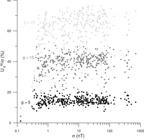
However, in addition to the relative standard uncertainty of the estimated mean, we are also interested in the relative
uncertainty at the level of confidence of 95%,U95
−g/σ; i.e.,
the relative error which will hardly ever be surpassed. A similar set of results applies in this case, whereby Fig. 8 is equivalent to Fig. 7 for the 95th percentile.
Again, U−95g/σ slightly increases with σ, although the
scatter overshadows this increment, maintaining it as rel-atively insignificant. In this case, the data are even more scattered than those of Fig. 7. Table 6 shows the central
68% interval of the distribution ofU95
−g/σ values for each
gap lengthgfrom 0 to 25 (5 by 5).
In order to illustrate the results, we can say we are
0.1 1 10 100 1000 (nT)
0 20 40 60 80
U-g
95/(
%
)
g = 25
g = 15
g = 5
Fig. 8. Equivalent to Fig. 7 for the 95th percentile case.
Table 6. Upper and lower limits of the central 68% accumulated probability forU−95g/σ. Values are percentages. Alternatively, this interval can be
understood as the standard uncertainty interval associated to the parameterU−95g/σ.
Gap lengthg→ 0 5 10 15 20 25
Upper and lower limit of the 68% central interval 0–0 12–17 23–31 31–44 37–57 43–70
ably confident (at the 95% level) that the mean computed with an absence of 5 running minutes will not be off the
actual mean by more than 0.14σ±0.02σ (see Table 6,
col-umn with headerg =5). The stated uncertainty (±0.02σ)
arises from the dependence of theU95
−g/σ on the
distribu-tion of the magnetic field values within the specific hourly interval considered, rather than on the observatory latitude or activity level itself, so that 68% of the analyzed hours
(i.e., 0.68×360 =245) have this 95% level within 0.02σ
around 0.14σ. Again, this differs from the case of random
extraction, where we had spot values forU95
−g/σ instead of
an interval.
The above results are based on analysing each individual hourly interval separately. The relative standard and 95% confidence level uncertainties are obtained for each hour, and the figures are based on the probability that a (new) hourly interval, with its particular number of missing data, has a certain value of uncertainty. Let us refer to it as the ‘individual’ approach. Nevertheless, we can go one step further by placing the statistics of all the stations and activ-ity levels together, i.e., the 360 analyzed hourly intervals. We will refer to this as the ‘simultaneous’ approach so as to differentiate it from the previous one. To a certain extent, we believe this to be an appropriate and correct approach since we have shown that the observatory or magnetic ac-tivity in question bear little, if any, influence on the results. Thus the new procedure will be:
(1) Consider all the possible ways of extractinggrunning
minutes from an individual hourly interval and
com-pute the different means, xh−,gi, where the h index
stands for the specific hourly interval andi for a
par-ticular extraction combination.
(2) Divide the differences between the estimated and
ac-tual means byσ (of that particular hour), so that the
relativedifferences (xh−,gi − xh0)/σh are obtained.
(3) Repeat this process for the 360 hours (h =1 to 360).
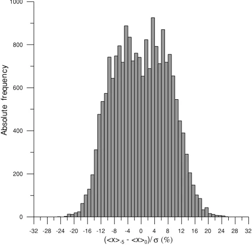
(4) Finally, we put all these relative differences together.
Thus, for a gap lengthg=5, a total of 360×(61−5)=
20160 relative differences are obtained, see Fig. 9. It is then straightforward to obtain the 95th percentile of this
distribu-tion. As well as this, the RMS−g/σ value is obtained from
Eq. (1) replacing (xi
−g − x0) with (x
h,i −g− x
h 0)/σ
h.
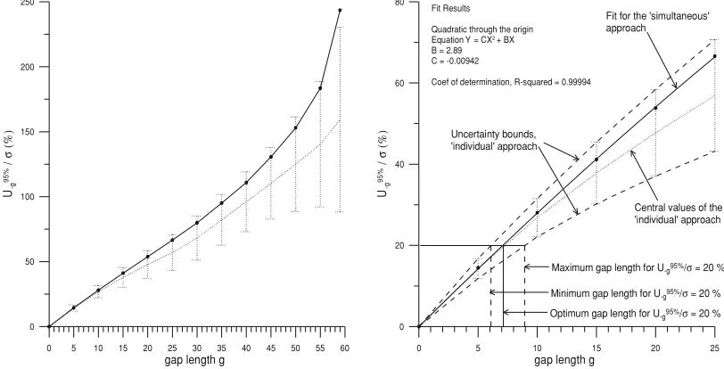
The results are summarized in Table 7 and Figs. 10 and 11. As seen in Fig. 10 for the relative standard uncertainty,
except forg = 59, the results of both methods (solid and
discontinuous lines) roughly coincide. The solid line in the right-hand part of Fig. 10 is a linear (through the origin) fit of the relative standard uncertainty obtained with the si-multaneous analysis method for small and moderate gap lengths. The empirical relationship between both magni-tudes is found to be:
RMS−g
σ ≈0.0158g (2)
The results from both methods are not so close for the case
ofU95
−g/σ (Fig. 11), especially forg >15. The solid line
in the right-hand part of Fig. 11 is a quadratic (through the
origin) fit ofU95
ap--32 -28 -24 -20 -16 -12 -8 -4 0 4 8 12 16 20 24 28 32
(<x>-5 - <x>0)/
0 200 400 600 800 1000
Abs
o
lut
e
freq
u
e
nc
y
Fig. 9. Distribution of the 20160 relative differences obtained as a result of a simultaneous analysis for the whole set of hourly intervals for a gap length
g=5.
Table 7. RMS−g/σandU−95g/σof the overall distribution of the relative differences for the 360 hourly intervals being studied after extraction of gap
segments of different lengths (simultaneous analysis). Values are percentages.
Gap lengthg→ 0 5 10 15 20 25
RMS−g/σof the global set 0 8.1 16 24 31 39
U−95g/σof the global set 0 14 28 41 54 67
proach for small and moderate gap lengths. The empirical relationship between both magnitudes is:
U95 −g
σ ≈0.0289g−0.0000942g2 (3)
Thus, for an hourly interval with a continuous gap segment of 6 minutes in length, which means 10% of the data is missing, the estimated mean will have a relative standard uncertainty of the order of 9% (result from Eq. (2)). Fur-thermore, we can be confident of our mean within a relative uncertainty of the order of 17% (result from Eq. (3)).
Finally, it may be of interest to note that a value for both the absolute root mean square, RMS, and 95% confidence
limit,U95, may be obtained by multiplying Eqs. (2) and (3)
byσ. Of course, we do not know the exact value of this
parameter when dealing with missing data (since it is de-fined for the complete data set), but to a first approximation
we can evaluateσ with the available data. Furthermore, it
is worth mentioning that it is probably meaningless to ob-tain a mean with an accuracy higher than the resolution the MHVs will finally be reported with. In this sense, care must
be taken when obtainingU95via Eq. (3) when dealing with
extremely quiet intervals.
2.3 Comparison between the random and continuous extraction approaches
A direct comparison of Tables 3 and 4 with Table 7 shows that the random extraction method is not appropriate for outlining the results of the MHV problem, since data are
unlikely to be missing in a randomly distributed way over a real hourly interval. One continuous gap is, by far, the most common way that minute values are absent. Cases with 2 gaps are the second most common situation (Schott and Linthe, 2007). A study of the number of gap segments per hour would yield slightly different results in each obser-vatory. Nevertheless, we can take the results for the EBR observatory as an orientation. The results show that a 1 gap segment (i.e., one continuous gap) has a 94% probability, while 2 gap segments account for virtually all the remain-ing 6% of cases. Thus, in a real situation the results for the uncertainties will be somewhere between those obtained in the two preceding subsections. In the following part we will try to find out how far this 6% can affect the results given in Section 2.2.
It is worth mentioning that, as expected, the uncertainty associated with a single gap is much greater than the uncer-tainty of randomly distributed gaps; thus, for a given num-ber of missing data, the estimated mean will be closer to the actual one in the latter case. Let us suppose that the assump-tion stated at the beginning of Secassump-tion 2 is a general rule: for a fixed number of missing data, long gaps (i.e., fewer seg-ments) are less reliable than short gaps (greater number of segments) when considering the mean computation.
Let us now consider the ‘simultaneous’ approach taken at the end of Section 2.2, for which the 20160 relative
dif-ferences for g = 5 are shown in Fig. 9. These
rela-0 5 10 15 20 25 30 35 40 45 50 55 60
gap length g
0 50 100 150 200 250
RM
S-g
/
0 20 40 60 80
RMS
-g
/
0 5 10 15 20 25
gap length g
Fit Results Linear through origin Equation Y = BX B = 1.58
Coef of determination, R-squared = 0.99996
Fig. 10. The left-hand graph shows the standard uncertainty of the relative differences after extraction of different gap lengthsg, whereas the right-hand plot shows a zoom for small and moderategvalues. Discontinuous lines show the distribution of the relative standard uncertainties and error bars on them bound the central 68% of analyzed hours (results from the ‘individual’ analysis); solid lines correspond to the standard uncertainty determination of the overall distribution of the relative differences (results from the ‘simultaneous’ analysis).
0 5 10 15 20 25 30 35 40 45 50 55 60
gap length g
0 50 100 150 200 250
U-g
95%
/
0 20 40 60 80
U-g
95
% /
0 5 10 15 20 25
gap length g
Fit Results
Quadratic through the origin Equation Y = CX2+ BX
B = 2.89 C = -0.00942
Coef of determination, R-squared = 0.99994
Maximum gap length for U-g95%/ = 20 %
Minimum gap length for U-g95%/ = 20 %
Optimum gap length for U-g95%/ = 20 %
Uncertainty bounds, 'individual' approach
Fit for the 'simultaneous' approach
Central values of the 'individual' approach
Fig. 11. Same as Fig. 10 for the relative 95% confidence level. Uncertainty bounds have been placed around the ‘individual’ approach central values, so as to include the 68% of the analyzed hourly intervals (i.e., 245). As an example, the correspondence between a particular value ofU−95g(20% of
σ) and its associated gap length (between 6 and 9, with a maximum probability corresponding to 7) is outlined.
Table 8. Maximum percentage reduction of the 95th percentile for a realistic gap segment distribution with respect to the 95th percentile obtained when considering only continuous gaps (Table 7).
Missing datag 0 5 10 15 20 25 30 35 40 45 50 55 59
% reduction 0 0.2 0.2 0.2 0.3 0.3 0.4 0.6 0.7 0.9 1.6 1.7 0.7
tive differences obtained with 2 (or more) gap segments in
the proportion 6/94 (=probability of 2 or more gap
seg-ments over 1 gap segment), the number will increase to
20160×100/94≈21447. The new 1288 added points will
be distributed in the histogram of Fig. 9. However, if we make the assumption stated in the previous paragraph, the corresponding relative differences will be closer to 0 than those of the continuous case, so they will accumulate in
the central part of the histogram. Computing the 95th per-centile of the new distribution involves rejecting the 5% of the cases corresponding to the greatest relative differences, which in the worst case will not affect the added points.
This means we must reject 0.05×21447=1072 points of
and more than one gap segments in adequate proportions) is equivalent to applying the 94.68th percentile to the distribu-tion of the continuous extracdistribu-tion case; obviously, the upper limit constitutes the former 95th percentile. Based on this, Table 8 summarizes the maximum reductions with respect
to the last row of Table 7, assuming that the proportion 6/94
is maintained for each number of missing data,g.
As seen, the reductions are imperceptible in most cases. The same can be seen even when the proportion of 2 or more gap segments is considerably greater than 6%, so we can take the results obtained for the continuous case (Table 7) as sufficiently good approximations, rather than those given in Tables 3 and 4.
3.
Conclusions and Future Work
The degree of accuracy of the MHVs is related to the (natural) magnetic variability of the respective hour. Thus, rather than using a fixed parameter, in our discussion we have referred to the standard deviation of the original data.
Our analysis set out to provide a general answer to the penultimate question posed in the introduction: When com-puting an MHV, what is the maximum number of missing data we can permit in an hourly interval, and still be
rea-sonably confident that the (pre-established) required
rela-tiveaccuracy is still achieved? The answer to this question
is not a simple figure and needs qualification. We analyzed a total of 360 hourly intervals from observatories at different latitudes and diverse magnetic activity levels, and we con-cluded that the answer depends principally on the particular distribution of the magnetic field values within the hourly interval, rather than on a specific observatory or magnetic activity at that time. This important fact allowed us to es-tablish a general rule roughly valid for any location and ac-tivity level; nevertheless, the mentioned dependence on a given distribution of the minute values within the hour gives rise to a certain ‘range of possible answers’ to the question posed above. In this sense, the uncertainty (corresponding to a confidence level of 95%) of the mean of our hourly interval in question, with a given amount of missing data, may fall within a finite interval. As the number of missing
data increases (g >25) the answer to our question becomes
increasingly vague, since the analyzed hours show increas-ingly disparate outcomes, or equivalently, the referred inter-val is too large for a practical purpose. However, the results presented for shorter gaps are quite consistent, and at least we have an order of magnitude for the uncertainty associ-ated to greater gaps
In this paper we provide some useful tools relating rel-ative accuracy and number of missing data. Thus, once a data user has established their required relative accuracy, our procedure provides a range for the maximum number of missing data to be permitted in the MHVs of their study. Let us consider the example of a data user requiring an er-ror in the estimated mean of, at most, 20% of the standard
deviation of the original data (i.e., 0.2σ). From our
anal-ysis, it is probable to obtain this result with a maximum number of missing data ranging from 6 to 9 minutes (this stems from the uncertainty bounds displayed in Fig. 11), depending, again, on variables which cannot be controlled
a priori, such as the particular distribution of the minute
values in each specific hourly interval. Given that the max-imum probability in this case is reached near 7 (Eq. (3) or Fig. 11 again), we suggest this figure as the optimum max-imum tolerable number of lost data in the hourly intervals of the analysis. In this way, it is easy to implement a simple algorithm which rejects hourly intervals with less than 53 minutes of data, ensuring (at the level of confidence of 95%) that its MHVs will not be off the true mean by more than 0.2 standard deviations of the original data set. As an alterna-tive to a self-computed threshold for each particular MHV user, if a general consensus is attained as regards the ‘av-erage’ relative accuracy required by data users, the IAGA association can establish a maximum number of missing data in the hourly intervals for computation of the observa-tories’ MHVs. Furthermore, as suggested in the last IAGA Workshop, it would even be possible to report an estimation of the standard uncertainty of each computed MHV; this
would be achieved by multiplying Eq. (2) by the σ value
obtained with the available data in each hourly interval.
Although X and H are the most widely-used magnetic
elements in modelling and magnetic field indexing, we
en-courage the undertaking of an analysis forY andZas well,
although similar results are expecteda priori.
Acknowledgments. The authors wish to thank the USGS for sup-plying the data from College, Boulder and San Juan observatories. They are also very grateful to Dr. L. F. Alberca, for his fruitful comments and suggestions. This work has been supported by Spanish project CGL2006-12437-C02-02/ANT of the Ministerio de Ciencia e Innovaci´on.
References
Green, P., Lunar and solar daily variations of the geomagnetic field at Toolangi,Pure Appl. Geophys.,101(1), 194–204, 1972.
ISO,Guide to the Expression of Uncertainty in Measurement, Geneva, Switzerland: International Organization for Standardization, 1993. Le Mou¨el, J., V. Kossobokov, and V. Courtillot, On long-term variations
of simple geomagnetic indices and slow changes in magnetospheric currents: The emergence of anthropogenic global warming after 1990?,
Earth Planet. Sci. Lett.,232(3–4), 273–286, 2005.
Mandea, M., 60, 59, 58, ... How many minutes for a reliable hourly mean?,
Proceedings of the Xth IAGA Workshop, Hermanus, 112–120, 2002. Martini, D. and K. Mursula, Correcting the geomagnetic IHV index of the
Eskdalemuir observatory,Ann. Geophys.,24(12), 3411–3419, 2006. Rangarajan, G. K., Some features of annual variation in the equatorial
geomagnetic field,Indian J. Radio Space Phys.,11, 152–155, 1982. Schott, J. J. and H. J. Linthe, The hourly mean computation problem
revisited,Proceedings of the XIIth IAGA Workshop, Belsk, 135–143, 2007.
Svalgaard, L. and E. W. Cliver, Interhourly variability index of geomag-netic activity and its use in deriving the long-term variation of solar wind speed,J. Geophys. Res.,112(A10), A10111, 2007.
Taylor, J. R.,An Introduction to Error Analysis. The study of Uncertainties in Physical Measurements, Oxford University Press, California, 1982. Torta, J. M., J. J. Curto, and P. Bencze, Behaviour of the quiet day
ionospheric current system in the European region,J. Geophys. Res.,
102(A2), 2483–2494, 1997.
Torta, J. M., L. R. Gaya-Piqu´e, J. J. Curto, and D. Altadill, An inspection of the long-term behaviour of the range of the daily geomagnetic field variation from comprehensive modelling,J. Sol. Atmos. Terr. Phys., doi: 101016/j.jastp.2008.06.006, 2008.
Walker, J. K., V. Y. Semenov, and T. L. Hansen, Synoptic models of high latitude magnetic activity and equivalent ionospheric and induced currents,J. Atmos. Terr. Phys.,59, 1435–1452, 1997.