Dynamics of a fourth order system of rational difference equations

R E S E A R C H

Open Access

Dynamics of a fourth-order system of rational

difference equations

Q Din

_{, MN Qureshi and A Qadeer Khan}

*_{Correspondence:}

[email protected] University of Azad Jammu and Kasmir, Muzaffarabad, Pakistan

Abstract

In this paper, we study the equilibrium points, local asymptotic stability of an equilibrium point, instability of equilibrium points, periodicity behavior of positive solutions, and global character of an equilibrium point of a fourth-order system of rational difference equations of the form

xn+1=

α

β

γ

, yn+1=

α

β

γ

,

n= 0, 1,. . ., where the parameters

α,

β

γ

α

β

γ

x–3,y0,y–1,y–2,y–3are positive real numbers. Some numerical examples are given to verify our theoretical results.

MSC: 39A10; 40A05

Keywords: system of rational difference equations; stability; global character

1 Introduction and preliminaries

The theory of discrete dynamical systems and difference equations developed greatly dur-ing the last twenty-five years of the twentieth century. Applications of difference equations also experienced enormous growth in many areas. Many applications of discrete dynam-ical systems and difference equations have appeared recently in the areas of biology, eco-nomics, physics, resource management, and others. The theory of difference equations occupies a central position in applicable analysis. There is no doubt that the theory of difference equations will continue to play an important role in mathematics as a whole. Nonlinear difference equations of order greater than one are of paramount importance in applications. Such equations also appear naturally as discrete analogues and as numeri-cal solutions of differential and delay differential equations which model various diverse phenomena in biology, ecology, physiology, physics, engineering and economics. It is very interesting to investigate the behavior of solutions of a system of higher-order rational dif-ference equations and to discuss the local asymptotic stability of their equilibrium points. Cinar [] investigated the periodicity of the positive solutions of the system of rational difference equations

xn+=



yn

, yn+= yn xn–yn–

.

Stević [] studied the system of two nonlinear difference equations

Kurbanli [] studied the behavior of positive solutions of the system of rational difference equations

Bajo and Liz [] investigated the global behavior of the difference equation

xn+= xn– a+bxn–xn

for all values of real parametersa,b.

Kalabuˆsić, Kulenović, and Pilav [] investigated the global dynamics of the following systems of difference equations:

xn+=

Kurbanli, Çinar, and Yalçinkaya [] studied the behavior of positive solutions of the system of rational difference equations

xn+=

Touafek and Elsayed [] studied the periodic nature and got the form of the solutions of the following systems of rational difference equations:

xn+=

Similarly, Touafek, and Elsayed [] studied the periodicity nature of the following systems of rational difference equations:

xn+=

Recently, Zhang, Yang, and Liu [] studied the dynamics of a system of the rational third-order difference equation

n= , , . . . , where the parametersα,β,γ,α,β,γand initial conditionsx,x–,x–,x–, y,y–,y–,y–are positive real numbers. This paper is a natural extension of [, ].

Let us consider an eight-dimensional discrete dynamical system of the form

xn+=f(xn,xn–,xn–,xn–,yn,yn–,yn–,yn–),

yn+=g(xn,xn–,xn–,xn–,yn,yn–,yn–,yn–),

(.)

n= , , . . . , wheref :I_×J_→Iandg:I_×J_{→Jare continuously differentiable}

func-tions andI,Jare some intervals of real numbers. Furthermore, a solution{(xn,yn)}∞n=–

of the system (.) is uniquely determined by initial conditions (xi,yi)∈I ×J for i∈ {–, –, –, }. Along with the system (.), we consider the corresponding vector map

F= (f,xn,xn–,xn–,xn–,g,yn,yn–,yn–,yn–). An equilibrium point of (.) is a point (x¯,¯y)

that satisfies

¯

x=f(x¯,x¯,x¯,x¯,y¯,y¯,y¯,y¯),

¯

y=g(x¯,x¯,x¯,x¯,y¯,y¯,y¯,y¯).

The point (x¯,¯y) is also called a fixed point of the vector mapF.

Definition . Let (x¯,y¯) be an equilibrium point of the system (.).

(i) An equilibrium point(x¯,¯y)is said to be stable if for everyε> , there existsδ>  such that for every initial condition(xi,yi),i∈ {–, –, –, }if



i=–(xi,yi) – (x¯,¯y)<δimplies(xn,yn) – (x¯,y¯)<εfor alln> , where · is

the usual Euclidean norm inR_.

(ii) An equilibrium point(x¯,¯y)is said to be unstable if it is not stable.

(iii) An equilibrium point(x¯,¯y)is said to be asymptotically stable if there existsη>  such that_i=–(xi,yi) – (x¯,y¯)<ηand(xn,yn)→(x¯,y¯)asn→ ∞.

(iv) An equilibrium point(x¯,¯y)is called a global attractor if(xn,yn)→(x¯,y¯)asn→ ∞.

(v) An equilibrium point(x¯,¯y)is called an asymptotic global attractor if it is a global attractor and stable.

Definition . Let (x¯,y¯) be an equilibrium point of the map

F= (f,xn,xn–,xn–,xn–,g,yn,yn–,yn–,yn–),

wheref andgare continuously differentiable functions at (x¯,y¯). The linearized system of (.) about the equilibrium point (x¯,y¯) is

where

To construct the corresponding linearized form of the system (.), we consider the fol-lowing transformation:

transformation (.) is given by

FJ(x¯,y¯) =

X is a fixed point of F.If all eigenvalues of the Jacobian matrix JF aboutX lie inside the¯ open unit disk|λ|< ,thenX is locally asymptotically stable¯ .If one of them has a modulus greater than one,thenX is unstable¯ .

Theorem .(Routh-Hurwitz criterion)

For real numbers a,a, . . . ,an,let

P(λ) =λn+aλn–+· · ·+an–λ+an. (.)

Consider the polynomial equation

We define the n matrices as follows:

The following statements are true:

(i) A necessary and sufficient condition for all of the roots of(.)to have a negative real part isdet(Hj) > forj= , , . . . ,n.

(ii) A necessary and sufficient condition for the existence of a root of(.)with a positive real part isdet(Hj) < for somej∈ {, , . . . ,n}.

2 Main results

Let (x¯,y¯) be an equilibrium point of the system (.), then forα>βandα>β, the system

(.) has the following five equilibrium points:

P= (, ), P= (A,B), P= (–A,B), P= (A, –B), P= (–A, –B), following results hold:

≤xn≤

Proof The results are obviously true form= . Suppose that results are true form=k≥,

≤αxk+

Theorem . For the equilibrium point P= (, )of Equation(.),the following results hold:

(i) Letα<βandα<β,then the equilibrium pointP= (, )of the system(.)is locally asymptotically stable.

(ii) Ifα>βorα>β,then the equilibrium pointP= (, )of the system(.)is unstable.

Proof (i) The linearized system of (.) about the equilibrium point (, ) is given by

and

The characteristic polynomial ofFJ(, ) is given by

P(λ) =λ–

β. Since all eigenvalues of the Jacobian matrixFJ(, ) about (, ) lie in an open unit dick|λ|< , the equilibrium point

(, ) is locally asymptotically stable.

(ii) It is easy to see that ifα>βorα>β, then there exists at least one rootλof Equation

of Equation(.)is unstable.

Proof The linearized system of (.) about the equilibrium pointPis given by

and

The characteristic polynomial ofFJ(P) is given by

P(λ) =λ–LMλ– LMλ– LMλ– LMλ– LMλ– LMλ–LM+ . (.) The roots of the characteristic polynomialP(λ) given in Equation (.) are given by

–, ±ι, ±√L√M.

It is sufficient to prove that any one of these roots has absolute value greater than one. For this, consider

Proof The proof is similar to Theorem ., so it is omitted.

The following theorem is similar to Theorem . of [].

(i) If(xk,yk)∈(, (αγ–β) 

₎×₍₍α–β γ )



_,∞_{),then(xn,yn)}∈_{(, (}α–β γ )



₎×₍₍α–β γ )

 _,∞_). (ii) If(xk,yk)∈((αγ–β)



_,∞₎×_{(, (}α–β γ )



_{),then(xn,yn)}∈₍₍α–β γ )



_,∞₎×_{(, (}α–β γ )

 _).

Theorem . The system(.)has no prime period-two solutions.

Proof Assume that (p,q), (p,q), (p,q), . . . is a prime period-two solution of Equation (.) such thatpi,qi=  andpi=qifori= , . Then, from the system (.), one has

p= αp

β+γ(qq), p=

αp

β+γ(qq), (.)

and

q= αq

β+γ(pp)

, q= αq

β+γ(pp)

. (.)

From (.) and (.), one haspi,qi=  fori= , . Which is a contradiction. Hence, the

system (.) has no prime period-two solutions.

Theorem . Letα<β andα<β,then the equilibrium point P= (, )of Equation

(.)is globally asymptotically stable.

Proof Forα<β andα<β, from Theorem ., (, ) is locally asymptotically stable.

From Theorem ., it is easy to see that every positive solution (xn,yn) is bounded,i.e.,

≤xn≤μ and ≤yn≤ν for all n= , , , . . . , where μ=max{x–,x–,x–,x} and

ν=max{y–,y–,y–,y}. Now, it is sufficient to prove that (xn,yn) is decreasing. From the

system (.), one has

xn+ =

αxn–

β+γynyn–yn–yn–

≤αxn–

β <xn–.

This implies thatxn+<xn–andxn+<xn+. Hence, the subsequences{xn+},{xn+},

{xn+},{xn+}are decreasing,i.e., the sequence{xn}is decreasing. Similarly, one has

yn+ =

αxn–

β+γynyn–yn–yn–

≤ αyn–

β

<yn–.

This implies thatyn+<yn–andyn+<yn+. Hence, the subsequences{yn+},{yn+},

{yn+},{yn+}are decreasing,i.e., the sequence{yn}is decreasing. Hence,limn→∞xn=

limn→∞yn= .

Theorem . Letα>β andα>β.Then,for a solution(xn,yn)of the system(.),the following statements are true:

(i) Ifxn→,thenyn→ ∞.

3 Examples

In order to verify our theoretical results and to support our theoretical discussions, we consider several interesting numerical examples in this section. These examples represent different types of qualitative behavior of solutions to the system of nonlinear difference equations (.). All plots in this section are drawn with mathematica.

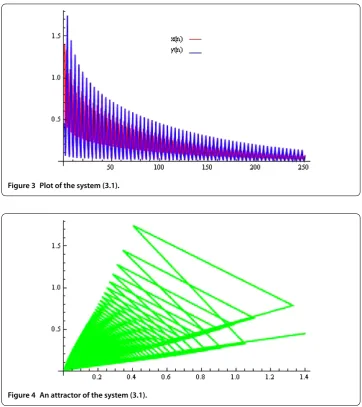
Example Consider the system (.) with initial conditionsx–= .,x–= .,x–= .,

x= .,y–= .,y– = .,y–= .,y= .. Moreover, choosing the parametersα=

.,β= .,γ = ,α= .,β= .,γ= , the system (.) can be written as

follows:

xn+=

.xn–

. + ynyn–yn–yn–

, yn+=

.yn–

. + xnxn–xn–xn–

, (.)

n= , , . . . , and with initial conditionsx–= .,x– = .,x–= .,x= .,y–= .,

y–= .,y–= .,y= .. The plot of the system (.) is shown in Figure  and its global

attractor is shown in Figure .

Figure 1 Plot of the system (3.1).

Figure 3 Plot of the system (3.1).

Figure 4 An attractor of the system (3.1).

Example Consider the system (.) with initial conditionsx–= .,x–= .,x–= ., x= .,y–= .,y–= .,y–= .,y= .. Moreover, choosing the parametersα= ,

β= .,γ = ,α= ,β= .,γ= , the system (.) can be written as follows:

xn+=

xn–

. + ynyn–yn–yn–

, yn+=

yn–

. + xnxn–xn–xn–

, (.)

n= , , . . . , and with initial conditionsx–= .,x–= .,x–= .,x= .,y–= .,

y–= .,y–= ., y= .. The plot of the system (.) is shown in Figure  and its global attractor is shown in Figure .

Example Consider the system (.) with initial conditionsx–= .,x–= .,x–= .,

x= .,y–= .,y–= .,y–= .,y= .. Moreover, choosing the parametersα=

,β = ,γ = ,α= ,β= ,γ= , the system (.) can be written as

follows:

xn+=

xn–

 + ynyn–yn–yn–

, yn+=

yn–

 + xnxn–xn–xn–

Figure 5 Plot of the system (3.3).

Figure 6 An attractor of the system (3.3).

n= , , . . . , and with initial conditionsx–= .,x–= .,x–= .,x= .,y–= .,

y–= .,y–= ., y= .. The plot of the system (.) is shown in Figure  and its global attractor is shown in Figure .

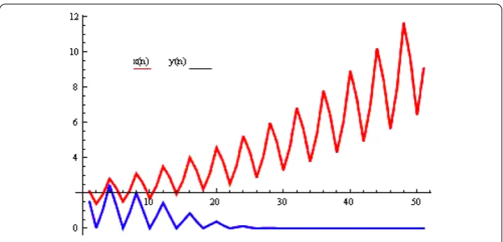
Example Consider the system (.) with initial conditionsx–= .,x–= .,x–= ., x= .,y–= .,y–= .,y–= .,y= .. Moreover, choosing the parametersα= ,

β= .,γ = ,α= ,β= ,γ= ., the system (.) can be written as follows:

xn+=

xn–

. + ynyn–yn–yn–

, yn+=

yn–

 + .xnxn–xn–xn–

, (.)

n= , , . . . , with initial conditionsx–= .,x–= .,x–= .,x= .,y–= .,y–=

.,y–= .,y= .. The plot of the system (.) is shown in Figure .

4 Conclusion

Figure 7 Plot of the system (3.4).

which except (, ) are unstable. The linearization method is used to show that the equilib-rium point (, ) is locally asymptotically stable. We prove that the system has no prime period-two solutions. The main objective of dynamical systems theory is to predict the global behavior of a system based on the knowledge of its present state. An approach to this problem consists of determining the possible global behaviors of the system and deter-mining which initial conditions lead to these long-term behaviors. In case of higher-order dynamical systems, it is crucial to discuss global behavior of the system. Some powerful tools such as semiconjugacy and weak contraction cannot be used to analyze global be-havior of the system (.). In the paper, we prove the global asymptotic stability of the equilibrium point (, ) by using simple techniques. Some numerical examples are pro-vided to support our theoretical results. These examples are experimental verifications of theoretical discussions.

Competing interests

The authors declare that they have no competing interests.

Authors’ contributions

QD and MNQ carried out the theoretical proof and drafted the manuscript. AQK participated in the design and coordination. All authors read and approved the final manuscript.

Acknowledgements

Authors would like to thank the referees for their comments and suggestions on the manuscript. This work was supported by the Higher Education Commission of Pakistan.

Received: 3 October 2012 Accepted: 3 December 2012 Published: 17 December 2012 References

1. Cinar, C: On the positive solutions of the difference equation systemxn+1=_yn1;yn+1=_xnyn

–1yn–1. Appl. Math. Comput.

158, 303-305 (2004)

2. Stevi´c, S: On some solvable systems of difference equations. Appl. Math. Comput.218, 5010-5018 (2012) 3. Kurbanli, AS: On the behavior of positive solutions of the system of rational difference equationsxn+1=_ynxnxn–1

–1 –1, yn+1=_xnynyn–1

–1 –1,zn+1= 1

ynzn. Adv. Differ. Equ.2011, 40 (2011)

4. Bajo, I, Liz, E: Global behaviour of a second-order nonlinear difference equation. J. Differ. Equ. Appl.17(10), 1471-1486 (2011)

5. Kalabuˆsi´c, S, Kulenovi´c, MRS, Pilav, E: Dynamics of a two-dimensional system of rational difference equations of Leslie–Gower type. Adv. Differ. Equ. (2011). doi:10.1186/1687-1847-2011-29

6. Kurbanli, AS, Çinar, C, Yalçinkaya, I: On the behavior of positive solutions of the system of rational difference equationsxn+1=_ynxnxn–1

–1 +1,yn+1=

yn–1

xnyn–1 +1. Math. Comput. Model.53, 1261-1267 (2011)

8. Touafek, N, Elsayed, EM: On the periodicity of some systems of nonlinear difference equations. Bull. Math. Soc. Sci. Math. Roumanie2, 217-224 (2012)

9. Zhang, Q, Yang, L, Liu, J: Dynamics of a system of rational third order difference equation. Adv. Differ. Equ. (2012). doi:10.1186/1687-1847-2012-136

10. Shojaei, M, Saadati, R, Adibi, H: Stability and periodic character of a rational third order difference equation. Chaos Solitons Fractals39, 1203-1209 (2009)

doi:10.1186/1687-1847-2012-215