R E S E A R C H
Open Access
Interference mitigation using random
antenna selection in millimeter wave
beamforming system
Woochang Lim
1, Girim Kwon
2*and Hyuncheol Park
2Abstract
In multi-user beamforming systems, the inter-user interference are controlled by spatial filtering. Since the implementation of digital beamforming is difficult due to high hardware cost of large array system, the analog beamforming system with one phase shifter at each antenna element is considered with antenna selection scheme. However, the beamwidth is not sufficiently narrow to perfectly remove the interference due to limited size of antenna arrays. To mitigate the interference, we propose the random antenna selection system in millimeter wave channel. The random antenna selection expands the effective array size so that the beamwidth becomes narrow. We compare the beamwidth of conventional fixed antenna selection with random antenna selection and analyze the amount of interference for each selection scheme. Theoretical analysis and bit error rate simulation results indicate that the beamforming with random antenna selection can take advantage of large array.
Keywords: Millimeter wave, Beamforming, Antenna selection, Large array
1 Introduction
Millimeter wave (mmWave) is one of the leading can-didates for the future wireless communications system thanks to the following two merits [1]. First, the large unlicensed bandwidth (30 to 300 GHz) allows us to solve the spectrum shortage. Second, the short wavelength of mmWave enables the devices to have a compact size with a lot of antenna elements. To utilize mmWave band, proper communication techniques suited for the channel charac-teristic should be employed. To this end, there are many mmWave-related standardization works such as European computer manufacturers association (ECMA)-387, IEEE 802.15.3c, IEEE 802.11ad, Wireless high-definition (Wire-lessHD), Next generation millimeter wave specification (NGmS), and Communication access long and medium range (CALM).
Since free-space path loss is proportional to frequency squared according to Friis equation, mmWave experi-ences more significant path loss than microwave below
*Correspondence: [email protected]
2School of Electrical Engineering, Korea Advanced Institute of Science and
Technology (KAIST), Daehak-ro 291, Daejeon 305-338, Republic of Korea Full list of author information is available at the end of the article
6 GHz [2]. Directional transmission such as beamforming is thus necessary because channel capacity and error rate depend on signal to noise ratio (SNR). Also, small wave length enables the achievement of high gain through syn-thesis of more antennas within limited area. However, the hardware complexity should be considered as the number of antenna elements are increased.
Maximal ratio transmission (MRT) is known as an optimal transmit beamforming technique where a domi-nant right singular vector of the channel matrix is used for precoding [3]. Unfortunately, high hardware com-plexity and cost make it difficult to implement MRT because it demands baseband digital signal processing (DSP) for each antenna element. For this reason, ana-log radio frequency (RF) beamforming is considered [4]. Equal gain transmission is one of the analog RF beam-forming schemes controlling only phase of signal with phase shifters [5, 6]. Also, analog-digital hybrid beam-forming techniques with the limited number of RF chains are considered to reduce the hardware complexity espe-cially in mmWave beamforming systems [7–10].
In single-user transmission system, a beamforming scheme for secure communication called antenna
set modulation (ASM) has been proposed in [11]. By selecting an antenna subset randomly for every symbol, ASM randomizes the amplitude and phase of received signal along a sidelobe. Although the original purpose of ASM is to average out the signals for undesired direc-tion by randomizadirec-tion, we can use the random antenna selection scheme to mitigate the inter-user interference in multi-user system which is considered in this paper. In multi-user transmission system, there exist many pre-coding techniques to suppress the inter-user interference. In [12], the codebook-based precoding with user schedul-ing algorithms has been proposed. In [13, 14], the linear methods such as block diagonalization precoding and non-linear methods such as Tomlinson-Harashima pre-coding are introduced. These techniques require a lot of RF chains to use DSP for each antenna element which results in high hardware complexity.
In this paper, we consider mmWave analog RF beam-forming system transmitting multiple streams simulta-neously with one phase shifter at each antenna element for low hardware complexity. Motivated by [11], we pro-pose the random antenna selection scheme for multi-user downlink system and analyze the amount of inter-user interference. We compare the performance of the random antenna selection with the conventional fixed antenna selection.
In the random antenna selection,Mantenna elements
are selected out of entire N antenna elements for each user. In the fixed antenna selection, on the other hand,M adjacent antenna elements are used for each user. There-fore, the effective aperture size of the random antenna selection for each user is larger than that of the fixed antenna selection. Since the beamwidth is proportional to the inverse of effective array size [15], the random antenna selection gives a narrower beamwidth. Finally, the interference with the signals for other users can be
mitigated. In the massive antenna array system, we can take advantage of large effective array size by random antenna selection.
The rest of this paper is organized as follows: in Section 2, the system model and channel model are described. The beamforming techniques with antenna selection are introduced in Section 3. We give the per-formance analysis for the conventional fixed antenna selection and the proposed random antenna selection in Section 4. The simulation results are provided in Section 5. The Conclusion follows in Section 6.
2 System description
In this section, we present our system model and chan-nel model. We consider multi-user MIMO system and mmWave channel.
2.1 System model
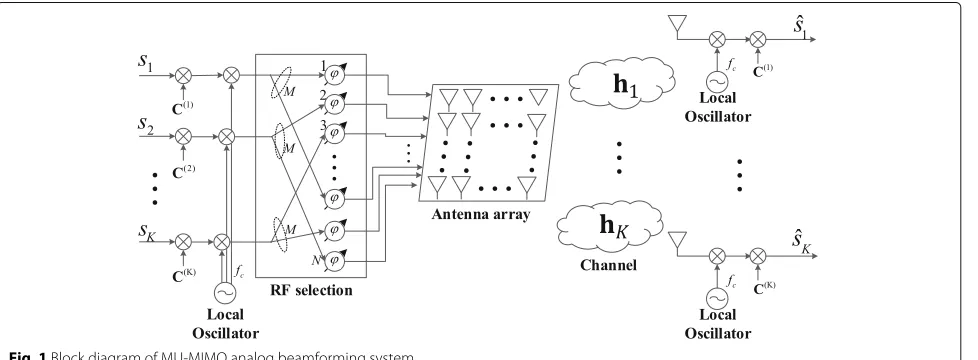
We consider a multi-user MIMO downlink system shown in Fig. 1. The base station (BS) has an antenna array with
N isotropic elements which have a unit gain, and each
user has a single antenna. The modulated symbols are multiplied by the spread code and transmitted by analog beamforming. We assume that the analog beamforming system controls the phase of transmitted signal with phase shifters, but cannot control the amplitude of the signals. In addition, each antenna element has only one phase shifter so that the system has low hardware complexity. There-fore,Kexclusive subsets of antenna elements are allocated to K RF chains to support a multi-user transmission. A spread code is used to separate the closely located users because they cannot be perfectly separated by beamform-ing techniques only. Since the finite number of antenna elements cannot provide sufficiently narrow beamwidth, a spread code is needed to distinguish the overlapped users. The spread symbol at chip timelwhich is represented by
xk[l] can be expressed as multiplication of the spread code C(k)[l] of lengthLwith the transmit symbolsk.
xk[l]=C(k)[l]sk. (1)
In our system, we assume that the BS has the infor-mation of angle of departures and corresponding path gains to compose the beamforming weight vectors. In order to obtain such channel state information (CSI) in mmWave beamforming system with the limited number of RF chains, two types of channel estimation techniques can be considered; closed loop estimation [16, 17] and open loop estimation [18]. For these channel estimation techniques, the beam training period is required to obtain the CSI. In the beam training period, the BS transmits a pilot beam pattern sequence to all users. After estimating the CSI using the pilot beam pattern sequence, each user feedbacks the estimated CSI to the base station for the purpose of transmit beamforming. Since multiple signals are transmitted simultaneously, the received signal for
usermcan be expressed by a summation of transmitted
signals for all users as follows.
rm[l]=hHm
K
k=1 wkxk[l]
+vm[l]
=hHm
K
k=1
wkC(k)[l]sk
+vm[l] , for 1≤l≤L,
(2)
wherehm ∈CN×1is channel vector for userm, andwk ∈
CN×1 is the beamforming vector for userkconsisted of
Mnon-zero complex numbers andN−Mzeros.M= NK
is the number of antenna elements allocated to each user. vm[l] is the complex Gaussian noise with zero mean and variance ofσ2.
After despreading, the received signal can be written as
ˆ rm=1
L L
l=1
C(m)[l]hHm
K
k=1
wkC(k)[l]sk
+1
L L
l=1
C(m)[l]vm[l]
=ρm,mhHmwmsm+ K
k=1 k=m
ρk,mhHmwksk+ ˜vm,
(3)
whereρk,m = 1L L
l=1
C(m)[l]C(k)[l]. We see that the
inter-ference can be mitigated by both spread code and beam-forming vectors. The more beambeam-forming mitigates the interference, the code lengthLcan be shorter.
The antenna array can be an arbitrary geometry such as linear array, rectangular array, cylindrical array, and spherical array. Since the antenna array has a sub-array
structure with K RF chains, it should be separated
into K exclusive subsets. We consider two methods for
antenna selection; fixed antenna selection and random antenna selection. These selection methods are presented in Section 3.
2.2 Channel model
In general, MIMO channel models can be separated into two categories. One is the physical model and the other is the analytical model [19]. In the physical models, we can express the physical propagation from transmit array and receive array by using the double-directional impulse response, h(t,τ,θt,φt,θr,φr), where t is the observed time,τ is the delay, and(θt,φt)and(θr,φr)are the (eleva-tion,azimuth) angles of departure and arrival, respectively [20]. We consider the double directional impulse response which is composed by the sum of the contributions from the discrete multi-path components, such that
ht,τ,θt,φt,θr,φr= ¯
N(t)
p=1 ¯
ρpejψpδ
τ −τp
δθt−θt p
×δφt−φt p δ
θr−θr
p δ
φr−φr
p ,
(4)
whereN¯ (t)is the number of multi-path components, and
βp ρ¯pejψp is the complex path gain. The superscripts
t and r correspond to the transmit and receive array,
respectively.
The double-directional model is useful because it is independent of the antenna array geometry. However, it is hard to theoretically analyze the system. Therefore, the analytical models are considered. These models describe the channel as a transfer function whose(i,j)entry is the transfer function from j-th transmit to the i-th receive antenna element. We can describe the channel transfer function matrix from the double-directional model. When
the BS has N antenna elements, and each ofK users is
equipped with a single antenna, the channel vector for user-kcan be written as follows:
hk=
¯
N
p=1 ¯
ρk,pejψk,pe−j2πfcτk,pat
θt
k,p,φkt,p , (5)
wherepis the index of paths, andfcis carrier frequency, and ψk,p ∈[ 0, 2π] is uniformly distributed phase, and at is N × 1 array steering vector. Also, we ignore the dependence ontbecause the block fading is assumed as usual.
shadow boundary due to small diffraction angle. Fur-thermore, the short wavelength causes the limited scat-tering which cannot make the Rayleigh scatscat-tering. As a result, the line of sight (LOS) component is dominant in mmWave channel. The measurement of LOS and non-line of sight (NLOS) component in urban outdoor mmWave channel is provided by [21]. Rappaport et al. [21] shows that there is no root-mean-square (RMS) delay spread for all LOS links in mmWave channel, and the LOS path has no resolvable multi-path. Finally, we can consider the first path of (5) as the LOS path and the others as NLOS paths. Then, we can separate the channel into a LOS component and(N¯ −1)NLOS components as follows:
hk= ¯ρk,LOSat
θt
k,LOS,φkt,LOS
+ ¯
N
p=2 ¯
ρk,pejψk,pe−j2πfcτk,pat
θt
k,p,φkt,p .
(6)
3 Beamforming with antenna selection
In this section, we introduce the beamforming techniques with antenna selection to form the multi-user transmis-sion. Because each antenna has a single phase shifter, a subset of antenna array provides only one beam. In other words, we need to separate the entire antenna array into K subsets, and consider two types of antenna selection schemes; conventional fixed antenna selection [22, 23]
and random antenna selection. After selecting K
sub-sets,Kweight vectors are constructed as the analog beam steering vectors with directions ofKusers.
The detail descriptions of the conventional fixed antenna selection and the proposed random antenna selection are presented in Section 3.2 and Section 3.3. In Section 4 and Section 5, we show that the random antenna selection mitigates the interference with signals for other users. Intuitively, this advantage comes from the fact that the effective array size of random antenna selec-tion scheme is larger than that of fixed antenna selecselec-tion. In other words, the beamwidth becomes narrow which decreases the amount of interference.
3.1 Effective array size and beamwidth
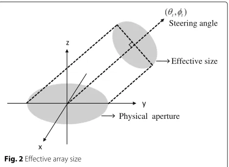
Although the spread code is used, the user-kcan be inter-fered with the signals for other users due to inaccurate synchronization or non-zero cross correlation between spread codes. The amount of interference is affected by the beamwidth overlapping with other user’s beam. The beamwidth is proportional to the inverse of effective array size which is dependent on the entire array size and steering angle [15]. The effective array size is the area of antenna array projected onto the perpendicular plane to the steering angle. The projected area is presented in Fig. 2. For example, for the linear array along with y-axis,
Fig. 2Effective array size
the effective array length becomesLcosθt, whereLis the actual array length, andθtis the steering angle.
3.2 Fixed antenna selection
When the antenna array is separated into K subsets, K
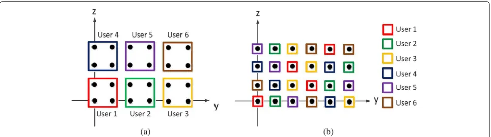
fixed patterns can be used to select the antenna elements, and each subset should be selected not to generate grating lobes which cause the strong interference with the signals for other users. Therefore, assuming that the antenna ele-ments are spaced at half wavelength, we have to select the adjacent elements to make a subset as [22, 23]. Otherwise, the grating lobes located at the fixed direction cause sig-nificant inter-user interference to certain users who are located at the same direction of the grating lobes. For example, for uniform planar array (UPA) placed on yz-plane, the fixed antenna selection patterns are presented in Fig. 3. In this case, the array steering vector for UPA is given by [15],
a(k)= ⎡ ⎢ ⎢ ⎢ ⎢ ⎢ ⎢ ⎢ ⎢ ⎢ ⎣
1 e−j2λπ(dzcosθ)
.. .
e−j2λπ(pdysinθsinφ+qdzcosθ) ..
.
e−j2λπ((Ny−1)dysinθsinφ+(Nz−1)dzcosθ) ⎤ ⎥ ⎥ ⎥ ⎥ ⎥ ⎥ ⎥ ⎥ ⎥ ⎦
, (7)
wherek=k0(sinθcosφ, sinθsinφ, cosθ)is wave vector, andk0= 2πλ is wave number, andλis wavelength. Assum-ing LOS dominant channel, each element of the weight vector for user-kis given by
wk(p,q)=
1 Mej
2π
λ(pdysinθksinφk+qdzcosθk) for(p,q)∈
k
0 for(p,q) /∈k
,
(8)
Fig. 3The fixed and random antenna selection patterns for uniform planar array :K=6.aFixed patterns.bRandom patterns
antenna elements along the y-axis(z-axis) such thatN = NyNz. Thedy(dz)is the uniform antenna spacing along the y-axis(z-axis). TheMis the number of antenna elements allocated to each user.k is the selected antenna subset for user-k. Then the beam pattern for user-kis obtained by inner product of array steering vector and weight vector as follows:
Bk(θ,φ)
= yk
1+My
y=yk 1
zk 1+Mz
z=zk 1
ej2λπ{ydy(sinθksinφk−sinθsinφ)+zdz(cosθk−cosθ)},
(9)
where (yk1,zk1) is the first element in k = {(yk1,zk1),
(yk1,z1k+1),· · ·,(yk1+My,zk1+Mz)}, andMyandMzare the number of elements along the y-axis and z-axis in a subset, respectively.
3.3 Random antenna selection
The other selection scheme considered in this paper is random selection. Every antenna element has same prob-ability to be chosen. To provide fairness to all users, the selection is changed at symbol rate. If the antenna array elements are selected arbitrarily, the grating lobes can be formed to undesired direction. However, we can average out the grating lobes by randomness in beam patterns. In addition, the beamwidth becomes narrow because the effective array size is larger than that of fixed antenna selection. As a result, the amount of interference with the signals for other users can be decreased.
Since the beam pattern for random antenna selection cannot be determined due to its randomness, it should be analyzed by statistical model. The analysis is derived in Section 4. Instead, the beam pattern which is averaged over 100 random beam patterns is chosen to be compared with the fixed antenna selection. In Fig. 4, the comparison of beam patterns are shown. The desired direction is set to be(θ,φ) =(120°,30°). The results show that the random
antenna selection gives narrower main lobes but higher side lobes than fixed antenna selection. Fortunately, since the LOS component is dominant in mmWave channel [11], the effect of increased level of side lobes which is still much lower than the level of main lobe is negligible. Therefore, the beamwidth of main lobe dominates the sys-tem performance. Note that the fixed antenna selection scheme with non-adjacent elements can also provide nar-rower beam than that with adjacent elements due to large effective array size. However, the antenna spacing which is larger than half-wavelength causes the grating lobes [15]. Due to the fixed position of the grating lobe, some other users who are located on the direction of the grating lobe may suffer from the significant interference. In the case of the random antenna selection scheme, on the other hand, the interference from random direction of the grat-ing lobes are averaged out so that other users who are located on different directions can receive their desired signals.
The random antenna selection can be implemented by sorting the long pseudo random sequence generated in
advance. First, we chooseN numbers from the sequence
generated by random number generator. After sorting the chosen numbers, we allocate theMnumbers to each user in consecutive order. On the other hand, the fixed antenna selection need not the sorting procedure. It only needs the consecutive sequence of lengthN to allocate the M numbers to each user in consecutive order. Once the ran-dom sequence (for ranran-dom selection) and consecutive sequence (for fixed selection) are generated, they can be used permanently. Therefore, the difference between ran-dom selection and fixed selection is time complexity of sorting procedure which is given byO(n2).
3.4 Discussion on the case of multiple paths
Fig. 4The normalized beam patterns for fixed and random antenna selection with uniform planar array:aFixed antenna selection withM= 4.b Fixed antenna selection withM= 16.cRandom antenna selection withM= 4.dRandom antenna selection withM= 16
analog architecture when there exist the multiple paths in mmWave channel.
First of all, we discuss the case of LOS channel. Since the BS transmits one symbol using the analog beamform-ing for each user, the BS cannot manage the inter-user interference. However, if two users are properly separated in their locations, the BS can distinguish the two users by making two directional beams. Nevertheless, it is still impossible to distinguish the two users when they are closely located to each other. For this case, the spread code is used for separating the closely located users. Here, the difference from the conventional code division mul-tiple access (CDMA) system is that the code length can be shorter than that of CDMA system due to the usage of beamforming technique.
In the case of multiple paths, the direction of the beamforming vector for each user is determined by the
dominant direction in the paths, i.e., LOS path. As we will discuss in Section 5, the path loss difference between LOS and NLOS links is quite large in millimeter wave chan-nel, e.g., 18 dB at 30 m and 21 dB at 50 m [21]. Although multiple paths exist, the effective difference of channel gains between LOS and NLOS links becomes much larger than the difference of path loss because of the beamform-ing gain. Therefore, the BS can mitigate the interference by means of both beamforming gain and spread code. The effect of the multiple paths on the performance is provided in Section 5.
4 Performance analysis
be easily applied to the uniform linear array (ULA)s or UPAs which are placed on arbitrary 1D line or 2D plane in the space. Note that sinceK beamforming vectors are constructed as the array steering vectors for the directions
ofK users, the system always guarantees the maximum
beam gain for the desired direction. On the other hand, the interference is affected by the side lobes of the beam pattern which depend on the antenna selection pattern. As a result, only the inter-user interference is affected by the introduced randomness, and the desired signal is not changed.
4.1 Null to null beamwidth
To compare the beamwidth of 3D beam patterns, we define(ux,uy,uz)space in terms of directional cosines,
uxsinθcosφ, uysinθsinφ, uzcosθ.
(10)
4.1.1 Fixed antenna selection
In the received signal (2), the weight vector can be expressed as
wherek is the selected antenna set for userk. The array steering vector is given by
at(θ,φ)= vector for each antenna element. The magnitude of beam
pattern can be obtained by the inner product of weight vector and steering vector,
Bk each axis in a subset. For each axis, the first null occurred at [15]
In the case of cuboidal array, we can express the null to null beamwidth for the fixed antenna selection as follows:
BWfixedNN = 2λ
If the antenna spacing is half-wavelength, (15) reduces to BWfixedNN = 64M.
4.1.2 Random antenna selection
selected or not. The mean magnitude of beam pattern for random antenna selection can be written as
EBk lar to the case of the fixed antenna selection, the null to null beamwidth for the random antenna selection with cuboidal array can be expressed as,
BWrandomNN = 2λ
If the antenna spacing is half-wavelength, (17) reduces to BWrandomNN = 64N.
From (15) and (17), we can see that the random antenna selection provides a narrower beamwidth than the fixed antenna selection at the rate of MN.
4.2 Interference analysis
We assume that the mmWave channel is dominated by LOS component as mentioned earlier. In Section 5, we see that the theoretical analysis can be applied to realistic mmWave channel. The normalized mmWave channel can be approximated as follows [11],
h=
4.2.1 Fixed antenna selection
To compare the interference between the two selection schemes, we first consider the fixed antenna selection scheme.
At the chip timel, the signal for user-ktransmitted from antenna element of position(x,y,z)can be written as
The interference with the signal for user-kaffecting user-mis represented byIk,m[l] as follows,
After despreading, the interference component in the received signal can be expressed as follows,
yk,m=
Eψk
where sk is expressed as √
Eseψk, and Es is the symbol energy, and ψk is the random variable representing the phase of the symbol for user-k.
The variance ofyk,mcan be expressed with two compo-nents; real part and imaginary part. The variances of each part can be found as
varReyk,m becomes zero, the total interference affecting user-mcan be expressed as follows,
K
4.2.2 Random antenna selection
For the random antenna selection, we can expressXx(k,y),z[l]
After despreading, the interference can be expressed as follows:
In contrast with the fixed antenna selection, each yk,m can be approximated as Gaussian random variable because it is the sum of bernoulli random variables.
First, we consider the randomness caused by random antenna selection for a given symbol. The mean of real part of (28) for a given symbol can be calculated as follows:
EZReyk,m|ψk
Similarly, the mean of imaginary part of (28) for a given symbol can be found as
The variances of real and imaginary part of (28) for a given symbol can be calculated as follows:
varReyk,m relation between real and imaginary part is calculated to obtain the covariance.
Using the second-order moment,EZ
(B) is calculated as follows:
(B)=ρ
covReyk,m
Now, we consider the randomness of symbol and
assume thatM-PSK is used for modulation scheme. All
symbols in the constellation have the same probability to be chosen. Therefore, the probability mass function of the random phase can be written as
Pr{ψk} =
21
P forψk=0,2πP ,· · ·, 2π(P−1)
P
0 otherwise , (37)
where thePis the modulation order. Taking the expecta-tion with respect to the symbol, we can obtain the mean and variance of interference. From (29) and (30), the mean of the interference can be found as
Eψk
From the relations in (29) and (31), the variance of real part is calculated as follows:
varReyk,m
In the same way, the variance of imaginary part also can be found from the relations in (30) and (32).
varImyk,m
From (36), the covariance between real and imaginary part is calculated as follows:
covReyk,m mean and variance ofyk,mare obtained as follows:
Eyk,m
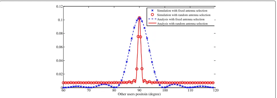
In (43), the second term comes from the randomness of each part ofyk,mfor givenψk, i.e., var[ Re{yk,m}|ψk] and var[ Im{yk,m}|ψk] as shown in (39) and (40). However, as other users’ positions are closer to the desired user, these randomness caused by random antenna selection can be ignored because of high correlation of received signals. In other words, as shown in Fig. 5, the randomness of antenna selection only appears in the region of side lobes, and there is no randomness in the region of main lobe. For this reason, in the case of highly correlated users, we have to ignore the effect of random selection in (43). For
example of ULA with N elements, since the phase
dif-ference between adjacent antenna elements is 2γk,m, the maximum phase difference from other antenna elements is(N −1)2γk,m. If(N −1)2γk,m is less thanπ, the sig-nals cannot be canceled to some extent but be reinforced by one-directional phases (either all positive phases or all negative phases). Since the terms related to the random selection are (31) and (32) which result in (39) and (40), we ignore Es(N−M)
60 70 80 90 100 110 120 0
0.02 0.04 0.06 0.08 0.1 0.12
Other users positoin (degree)
Simulation with fixed antenna selection Simulation with random antenna selection Analysis with fixed antenna selection Analysis with random antenna selection
Fig. 5The variance of total interference to a user located at 90o:M=12,K=6
yk,m∼CN
⎛ ⎝0,ρ
2 k,mEs
N2
sin(Nxαkm) sin(αkm)
2sinNyβ
km
sin(βkm)
2
sin(Nzγkm) sin(γkm)
2
+Tk,m
Es(N−M)
MN ρ
2 k,m
,
(44)
where
Tk,m
=
0 for|(Nx−1)2αkm|≤πandNy−1
2βkm≤πand|(Nz−1)2γkm|≤π
1 otherwise ,
(45)
and the total interference affecting user-m can be
expressed asKk=1 k=m
yk,m.
In Fig. 5, we verify the mathematical results in (25) and (44) with simulations by assuming ULA. We can see that the random antenna selection provides a narrower beamwidth than the fixed antenna selection. In other words, the random antenna selection has lower interfer-ence than the fixed antenna selection in the range of 83o ∼ 97o. This result implies that the random antenna selection mitigates the inter-user interference where the interference cannot be managed effectively by beamform-ing. Also, the random antenna selection can provide the fairness by reducing the interference to closer users and
by allowing a small amount of interference to farther users who can be tolerant of the interference. As a result, the random antenna selection mitigates the user inter-ference, and this is directly related with the beamwidth analysis in (15) and (17).
4.3 Bit error rate
Assuming that QPSK is used for the modulation scheme, the expressions for theoretical bit error rate (BER) for fixed antenna selection is given by,
Pfixedb
=Q
d
2σ
=Q
3
Eb N0
2 +
PI
2
=Q
⎛ ⎜ ⎜ ⎜ ⎝ 4 5 5 5 6
1
N0
2Eb+
1
M2 K
k=1
k=mρ
2
k,m sin(M
xαkm)
sin(αkm)
2sin(Myβkm) sin(βkm)
2sin(M
zγkm)
sin(γkm)
2
⎞ ⎟ ⎟ ⎟ ⎠,
(46)
where the interference is considered as noise, and PI andN0are the total interference power and noise power,
respectively, and d = 2√Eb is the minimum distance
of QPSK, and Eb is the bit energy. Theoretical BER for random antenna selection can be obtained as
Prandomb =Q
⎛ ⎜ ⎜ ⎜ ⎝
4 5 5 5 6
1
N0 2Eb +
K
k=1 k=m
2
ρ2 k,m
N2
sin(Nxαkm) sin(αkm)
2sin(N yβkm) sin(βkm)
2sin( Nzγkm) sin(γkm)
2
+Tk,m(NMN−M)ρk2,m
) ⎞ ⎟ ⎟ ⎟
uy
uz
−1 −0.8 −0.6 −0.4 −0.2 0 0.2 0.4 0.6 0.8 1 −1
−0.8 −0.6 −0.4 −0.2 0 0.2 0.4 0.6 0.8 1
0 0.1 0.2 0.3 0.4 0.5 0.6 0.7 0.8 0.9 1
Fig. 6Contour plot of magnitude of beam pattern for fixed antenna selection with UPA :M=16,K=6
5 Simulation results
In this section, we give the simulation results for the beamwidth comparison and BER performances. In our simulations, we focus on the effect of the random antenna selection in the system with onlyKRF chains as described in Fig. 1. Therefore, we compare the performances of the proposed random antenna selection with the fixed antenna selection which is conventional in the system with sub-array beamforming structure [22, 23].
5.1 Beamwidth
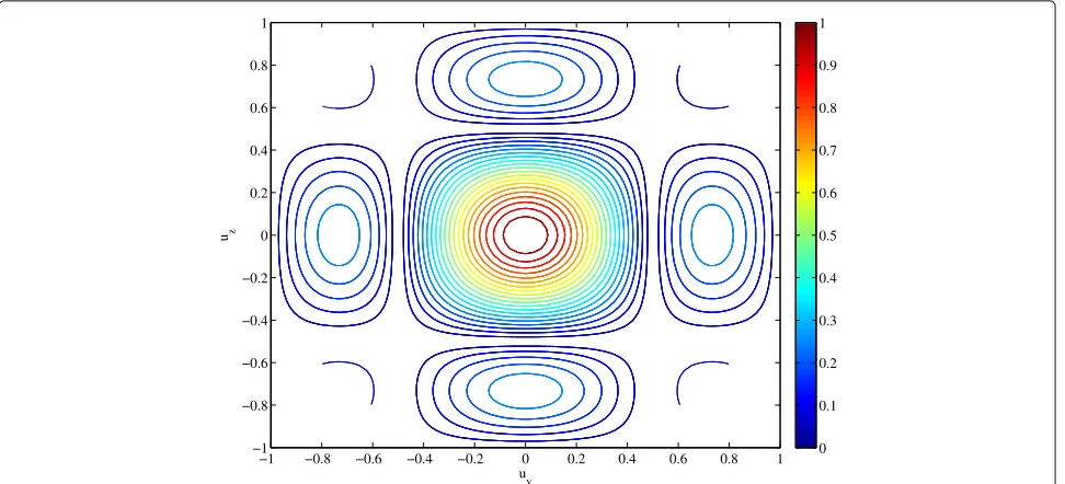
In the simulations, we assume that the UPA is placed on yz-plane, and the array is steered to(θ,φ)=(90°,0°), and K = 6,My = 4,Mz = 4,Ny = 12,Nz = 8,dy =
dz = λ/2. Figure 6 and 7 show the magnitude
con-tour of beam patterns in(uy,uz)space. We can see that the random antenna selection gives narrower beamwidth than fixed antenna selection, and the theoretical null-to-null beamwidth (15) and (17) are well matched with the
uy
uz
−1 −0.8 −0.6 −0.4 −0.2 0 0.2 0.4 0.6 0.8 1 −1
−0.8 −0.6 −0.4 −0.2 0 0.2 0.4 0.6 0.8 1
0 0.1 0.2 0.3 0.4 0.5 0.6 0.7 0.8 0.9 1
simulation results. The first null points for fixed antenna selection occurred atuy= ±12anduz= ±12, which results in BWfixedNN = 1. On the other hand, the first null points for random antenna selection occurred atuy = ±16 and uz = ±14, which results in BWrandomNN = 16. Therefore, the null-to-null beamwidth for random antenna selection is six times as narrow as that for fixed antenna selection. We can see that the area of main lobes in Fig. 6 is about six times as large as that in Fig. 7. From the results, we can infer that the random antenna selection can reduce the interference with the signals for other users.
5.2 Bit error rate
In the simulations, we assume that user-1 is located at
(θ,φ) =(90°,0°), and other users are located at the posi-tions with some offset degrees from user-1. The UPA lied on theyz-plane withdy = dz = λ/2 is used. The num-ber of multi-path components is set to beN¯ =30, and we use Gold code of length 15 for spread code and QPSK for modulation scheme. The transmitted power for each user is normalized to unity. The number of users is set to be K = 14, and the users are located with uniform offset of 2° in both elevation and azimuth angle. From the expres-sion in (46) and (47), the theoretical BER for user-1 can be calculated as follows:
Pfixedb
=Q
⎛ ⎜ ⎝
4 5 5
6 1
N0 2Eb +
1 225M2
14
k=2
sin(M yβk1) sin(βk1)
2sin( Mzγk1) sin(γk1)
2
⎞ ⎟
⎠,
(48)
Prandomb
=Q
⎛ ⎜ ⎜ ⎜ ⎝ 4 5 5 5 6
1
N0
2Eb+
1 225N2
14
k=2
2sin(N yβk1)
sin(βk1)
2sin(N
zγk1)
sin(γk1)
2
+13NTk,1
) ⎞ ⎟ ⎟ ⎟ ⎠.
(49)
First, we consider the LOS only channel in order to ver-ify the theoretical analysis. In Fig. 8,ρLOSis set to be 1 so that the channel is normalized to unity, and NLOS path does not exist. We can see that the random selection has
SNR gain of 2.5 dB for M = 16, and 4 dB forM = 4
at BER of 10−4. The smaller the number of antenna ele-ments, the larger the SNR gain becomes. Intuitively, the difference of effective array size between random selec-tion and fixed selecselec-tion forM = 4 is larger than that for
M = 16. Note that the performance differences between
M = 4 andM = 16 are from the beamforming gain due
to the number of total antenna elements. Also, we can see
0 2 4 6 8 10 12 14
10−5 10−4 10−3 10−2 10−1
BER for user−1
Random (M=4) Fixed (M=4) Random (M=16) Fixed (M=16) Random (theory) Fixed (theory)
Fig. 8BER for user-1 in LOS only channel
that the theoretical BER curves are well matched with the simulated curves. In contrast with random selection, the number of random variables summed together (K=14) is not large enough in the fixed selection which gives a slight inaccuracy.
Now, we provide the BER simulation in mmWave chan-nel model including the NLOS links. In [21], the urban outdoor mmWave channel measurements of time delay spread and path loss are provided for 38 and 60 GHz chan-nel. For 38 GHz channel, the path loss difference between LOS and NLOS links is 18 dB at 30 m and 21 dB at 50 m from transmitter. The 60 GHz channel also has similar behavior with 38 GHz. The LOS path has no resolvable multi-path, and the mean of RMS delay spread for NLOS link is 23.6 ns for 38 GHz and 7.4 ns for 60 GHz, and the maximum RMS delay spread for NLOS link is 122 ns for 38 GHz and 36.6 ns for 60 GHz. We can see that the delay spread for mmWave is very small especially for 60 GHz. To understand the effect of NLOS power, we assume that the number of resolvable path of NLOS is one which results inτp= ¯τrms. Considering the 38 GHz channel,τ¯rmsis set to be 23.6 ns. Figure 9 shows the effect of NLOS power,
where M = 16. When the path loss difference between
LOS and NLOS links is larger than 16 dB, the BER per-formance becomes almost the same with the LOS only channel. Since the path loss difference between LOS and NLOS links in mmWave is larger than 16 dB at more than 30 m [21], our theoretical analysis of LOS only channel can be accurately applied to the realistic mmWave channel. Moreover, we can infer that the random antenna selection has better performance than the fixed antenna selection even if the NLOS power becomes strong.
two-0 2 4 6 8 10 12 14 10−5
10−4 10−3 10−2 10−1
BER for user−1
Random (12dB) Fixed (12dB) Random (14dB) Fixed (14dB) Random (16dB) Fixed (16dB) Random (LOS only) Fixed (LOS only)
Fig. 9BER for user-1 in mmWave channel for different NLOS power
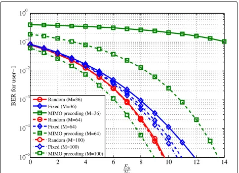
stage beamforming technique [24] is applicable. In the first stage, we use the same beamforming vectors with the fixed selection scheme to consider the sub-array structure. Assuming that the effective channel which is the prod-uct of the channel matrix and the RF beamforming matrix is known at the transmitter, the baseband beamforming matrix is constructed as zero-forcing precoder at the sec-ond stage. We assume the same simulation parameters with Fig. 8 except for the number of antennas. We see that the antenna selection schemes with spreading code outperform the hybrid beamforming scheme when the
total number of antennasN is equal toMK = 504 or
MK =896. In case ofMK=1400, the hybrid
beamform-ing scheme outperforms the antenna selection schemes. Since it is not easy to implement a thousand of anten-nas in practical systems, the antenna selection scheme with spreading code is more attractable than the hybrid beamforming scheme in terms of BER performance at the expense of time resources.
0 2 4 6 8 10 12 14
10−5 10−4 10−3 10−2 10−1 100
BER for user−1 Random (M=36)Fixed (M=36) MIMO precoding (M=36) Random (M=64) Fixed (M=64) MIMO precoding (M=64) Random (M=100) Fixed (M=100) MIMO precoding (M=100)
Fig. 10BER comparison with digital-analog hybrid precoding scheme
0 2 4 6 8 10 12 14
10−6 10−5 10−4 10−3
BER for user−1
Random (simulation) Fixed (simulation) Random (theory) Fixed (theory)
Fig. 11BER for user-1 versus user distribution with UPA :M=16,
K=14,Eb/N0=8 dB
In addition, we consider the effect of the position distri-bution of users. Figure 11 shows the BER versus user dis-tribution for UPA. We can see that the advantage of ran-dom antenna selection becomes large when other users are located near the user-1. If the positions of other users are far from the user-1, the performance gap becomes small. The results for ULA is provided in Fig. 12. In con-trast with UPA which conduct 3D beamforming, the ULA on z-axis cannot distinguish the azimuth angles. There-fore, the random antenna selection with ULA has smaller performance gain than that with UPA.
6 Conclusions
In this paper, we have proposed the random antenna selection scheme to mitigate the inter-user interference in multi-user mmWave beamforming systems. The prime advantage of this scheme is that it expands the effective array size to make a narrow beamwidth which reduces
0 2 4 6 8 10 12 14
10−4 10−3 10−2
BER for user−1
Random (simulation) Fixed (simulation) Random (theory) Fixed (theory)
Fig. 12BER for user-1 versus user distribution with ULA :M=16,
the overlapped area between the beams for each user. The beamwidth of the random antenna selection is MN times as narrow as the beamwidth of the conventional fixed antenna selection. We analyze the amount of interference for each selection scheme using Gaussian approximation and compare it with the simulation results in realistic mmWave channel. The advantage of random antenna selection can be well applied to mmWave 3D beamform-ing systems usbeamform-ing massive antenna array.
Acknowledgements
This research was supported by Basic Science Research Program through the National Research Foundation of Korea(NRF) funded by the Ministry of Science, ICT & Future Planning(2017R1A2B4009853). This work was also supported by the Institute for Information & communications Technology Promotion (IITP) grant funded by the Korea government (MSIP) (2017-0-00765).
Competing interests
The authors declare that they have no competing interests.
Publisher’s Note
Springer Nature remains neutral with regard to jurisdictional claims in published maps and institutional affiliations.
Author details
1Agency for Defense Development (ADD), P.O. Box 35, Daejeon 305-600,
Republic of Korea.2School of Electrical Engineering, Korea Advanced Institute
of Science and Technology (KAIST), Daehak-ro 291, Daejeon 305-338, Republic of Korea.
Received: 24 April 2015 Accepted: 21 April 2017
References
1. SK Yong, CC Chong, An overview of multigigabit wireless through millimeter wave technology: potentials and technical challenges. EURASIP J. Wirel. Commun. Netw.2007(078907) (2006). doi:10.1155/2007/78907 2. Z Pi, F Khan, An introduction to millimeter-wave mobile broadband
systems. IEEE Commun. Mag.49(6), 101–107 (2011)
3. DJ Love, RW Heath, T Strohmer, Grassmannian beamforming for multiple-input multiple-output wireless systems. IEEE Trans. Inform. Theory.49(10), 2735–2747 (2003)
4. J Wang, Z Lan, C Pyo, T Baykas, C Sum, M Rahman, J Gao, R Funada, F Kojima, H Harada, et al., Beam codebook based beamforming protocol for multi-Gbps millimeter-wave WPAN systems. IEEE J. Sel. Areas Commun.27(8), 1390–1399 (2009)
5. S-H Tsai, Equal gain transmission with antenna selection in MIMO communication. IEEE Trans. Wireless Commun.10(5), 1470–1479 (2011) 6. DJ Love, RW Heath, Equal gain transmission in multiple-input
multiple-output wireless systems. IEEE Trans. Commun.51(7), 1102–1110 (2003)
7. OE Ayach, S Rajagopal, S Abu-Surra, Z Pi, RW Heath, Spatially sparse precoding in millimeter wave MIMO systems. IEEE Trans. Wireless Commun.13(3), 1499–1513 (2014)
8. G Kwon, Y Shim, H Park, HM Kwon, in2014 IEEE 80th Vehicular Technology Conference (VTC2014-Fall). Design of millimeter wave hybrid
beamforming systems (IEEE, Vancouver, 2014), pp. 1–5. doi:10.1109/VTCFall.2014.6965933
9. G Kwon, H Park, in2015 IEEE Global Communications Conference (GLOBECOM). An efficient hybrid beamforming scheme for sparse millimeter wave channel (IEEE, San Diego, 2015), pp. 1–6. doi:10.1109/GLOCOM.2015.7417344
10. TE Bogale, LB Le, A Haghighat, L Vandendorpe, On the number of RF chains and phase shifters, and scheduling design with hybrid analog-digital beamforming. IEEE Trans. Wireless Commun.15(5), 3311–3326 (2016)
11. N Valliappan, A Lozano, RW Heath, Antenna subset modulation for secure millimeter-wave wireless communication. IEEE Trans. Commun.61(8), 3231–3245 (2013)
12. BM Lim, K Ahn, H Kim, H Park, GT Gil, in2010 IEEE 71st Vehicular Technology Conference. Improved user scheduling algorithms for codebook based MIMO precoding schemes (IEEE, Taipei, 2010), pp. 1–5.
doi:10.1109/VETECS.2010.5493763
13. QH Spencer, AL Swindlehurst, M Haardt, Zero-forcing methods for downlink spatial multiplexing in multiuser MIMO channels. IEEE Trans. Signal Process.52(2), 461–471 (2004)
14. C Windpassinger, RFH Fischer, T Vencel, JB Huber, Precoding in multi-antenna and multi-user communications. IEEE Trans. Wireless Commun.3(4), 1305–1316 (2004)
15. HLV Trees,Optimum array processing: part IV of detection, estimation, and modulation theory. (Wiley-Interscience, New York, 2002)
16. S Hur, T Kim, DJ Love, JV Krogmeier, TA Thomas, A Ghosh, Millimeter wave beamforming for wireless backhaul and access in small cell networks. IEEE Trans. Commun.61(10), 4391–4403 (2013)
17. A Alkhateeb, OE Ayach, G Leus, RW Heath, Channel estimation and hybrid precoding for millimeter wave cellular systems. IEEE J. Sel. Top. Signal Process.8(5), 831–846 (2014)
18. J Lee, G-T Gil, YH Lee, in2014 IEEE Global Communications Conference. Exploiting spatial sparsity for estimating channels of hybrid MIMO systems in millimeter wave communications (IEEE, Austin, 2014), pp. 3326–3331. doi:10.1109/GLOCOM.2014.7037320
19. P Almers, E Bonek, A Burr, N Czink, M Debbah, V Degli-Esposti, H Hofstetter, P Kyö, D Laurenson, G Matz, et al., Survey of channel and radio propagation models for wireless MIMO systems. EURASIP J. Wirel. Commun. Netw. 20072007(019070) (2007). doi:10.1155/2007/19070 20. M Steinbauer, AF Molisch, E Bonek, The double-directional radio channel.
IEEE Antennas Propag. Mag.43(4), 51–63 (2001)
21. TS Rappaport, E Ben-Dor, JN Murdock, Y Qiao, in2012 IEEE International Conference on Communications (ICC). 38 GHz and 60 GHz
angle-dependent propagation for cellular & peer-to-peer wireless communications (IEEE, Ottawa, 2012), pp. 4568–4573.
doi:10.1109/ICC.2012.6363891
22. OE Ayach, RW Heath, S Rajagopal, Z Pi, in2013 IEEE Global Communications Conference (GLOBECOM). Multimode precoding in millimeter wave MIMO transmitters with multiple antenna sub-arrays, (2013), pp. 3476–3480. doi:10.1109/GLOCOM.2013.6831611 23. W Roh, JY Seol, J Park, B Lee, J Lee, Y Kim, J Cho, K Cheun, F Aryanfar,
Millimeter-wave beamforming as an enabling technology for 5G cellular communications: theoretical feasibility and prototype results. IEEE Commun. Mag.52(2), 106–113 (2014). doi:10.1109/MCOM.2014.6736750 24. A Alkhateeb, G Leus, RW Heath, Limited feedback hybrid precoding for
multi-user millimeter wave systems. IEEE Trans. Wireless Commun.14(11), 6481–6494 (2015)
Submit your manuscript to a
journal and benefi t from:
7 Convenient online submission
7 Rigorous peer review
7 Immediate publication on acceptance
7 Open access: articles freely available online
7 High visibility within the fi eld
7 Retaining the copyright to your article