R E S E A R C H
Open Access
A new spline in compression method of
order four in space and two in time based on
half-step grid points for the solution of the
system of 1D quasi-linear hyperbolic partial
differential equations
RK Mohanty
1*and Gunjan Khurana
1,2*Correspondence:
[email protected] 1Department of Applied
Mathematics, South Asian University, Akbar Bhawan, Chanakyapuri, New Delhi, 110021, India
Full list of author information is available at the end of the article
Abstract
In this paper, we propose a new three-level implicit method based on a half-step spline in compression method of order two in time and order four in space for the solution of one-space dimensional quasi-linear hyperbolic partial differential equation of the formutt=A(x,t,u)uxx+f(x,t,u,ux,ut). We describe spline in compression
approximations and their properties using two half-step grid points. The new method for one-dimensional quasi-linear hyperbolic equation is obtained directly from the consistency condition. In this method we use three grid points for the unknown functionu(x,t) and two half-step points for the known variable ‘x’ inx-direction. The proposed method, when applied to a linear test equation, is shown to be
unconditionally stable. We have also established the stability condition to solve a linear fourth-order hyperbolic partial differential equation. Our method is directly applicable to solve hyperbolic equations irrespective of the coordinate system, which is the main advantage of our work. The proposed method for a scalar equation is extended to solve the system of quasi-linear hyperbolic equations. To assess the validity and accuracy, the proposed method is applied to solve several benchmark problems, and numerical results are provided to demonstrate the usefulness of the proposed method.
MSC: 65M06; 65M12
Keywords: spline in compression approximations; quasi-linear hyperbolic equations; half-step grid points; telegraphic equation; unconditionally stable; maximum absolute errors
1 Introduction
We consider a one-space dimensional quasi-linear hyperbolic equation of the type
utt=A(x,t,u)uxx+f(x,t,u,ux,ut), <x< ,t> , (.)
with the following initial conditions:
u(x, ) =p(x), ut(x, ) =q(x), ≤x≤, (.)
and boundary conditions
u(,t) =r(t), u(,t) =r(t), t≥. (.)
We assume that the functionsA(x,t,u) andu(x,t) are sufficiently smooth, the required higher order partial derivatives ofA(x,t,u) andu(x,t) exist in the solution domain≡ {(x,t)| <x< ,t> }, and the conditions (.) and (.) are given with sufficient smooth-ness to maintain the order of accuracy in the numerical method under consideration. Further, we assume that the initial and boundary value problem (.)-(.) has a unique smooth solutionu(x,t) in the solution domain. The details of existence and uniqueness of the above initial boundary value problem have already been discussed in [].
A wave is a time evolution phenomenon that we generally model mathematically using partial differential equations (pdes) which have a dependent variableu(x,t), which repre-sents the wave value, an independent variable, timetand one or more independent spatial variables. The actual form that the wave takes is strongly dependent upon the system’s ini-tial conditions, boundary conditions and disturbances in the system.
Wave equation is an important second-order linear partial differential equation for the description of waves as they occur in real life such as ripples on a lake, wind waves on water, tidal surges in estuaries, transverse waves travelling on a long string, transverse vibrations of strings and membranes, traffic density waves, seismic waves, acoustic waves and electromagnetic wave currents in coaxial cables.
Problems involving the propagation of nonlinear waves have become of increasing in-terest in various branches of science and engineering. In general, waves of finite ampli-tude governed by a nonlinear evolution equation are called nonlinear waves. As is well known, the principle of superposition of solutions is not valid in nonlinear equations. Therefore the methods familiar to physicists and engineers, like the use of Fourier or Laplace transforms, are no longer applicable with the result that the study of nonlinear waves has not yet become well established. However, in recent years, a number of inter-esting phenomena involving nonlinear waves have been found, and with the development of digital computers remarkable progress has been made in the research into nonlinear waves.
[] discussed a cubic spline method for solving singular two-point boundary value prob-lems. Mohantyet al.[–] gave spline in compression methods for singularly perturbed two-point singular boundary value problems and gave convergent spline in tension meth-ods for singularly perturbed two-point singular boundary value problems. Rashidineaet al.[, ] discussed spline methods for the solution of hyperbolic and parabolic equa-tions. Islam et al.[, ] studied non-polynomial spline approximations for the solu-tion of boundary value problems. Ding and Zhang [] studied parametric spline meth-ods for the solution of hyperbolic equations. Mohanty and Jain [] studied the use of a cubic spline method for the solution of D quasilinear parabolic equations. Recently, Mohantyet al.[, ] derived numerical methods based on non-polynomial spline ap-proximations for the solution of D quasilinear hyperbolic equations. In these methods, they have used full-step grid points, hence these methods are not directly applicable to problems in polar coordinates. Mohantyet al.[–] have also used different techniques for the solution of one-dimensional nonlinear wave equations. Most recently, Mohanty and Khurana [] have proposed a high accuracy numerical method based on off-step discretization for the solution of D quasilinear hyperbolic equations. To the authors’ knowledge, no numerical method based on half-step spline in compression approxima-tion has been developed for the one-dimensional quasi-linear hyperbolic equaapproxima-tion from the consistency condition so far. In this paper, we propose a method derived from the con-sistency condition, which is applicable to hyperbolic equations irrespective of coordinate systems.
Our paper is arranged as follows. In Section , we discuss the properties of spline in compression approximations. In Section , we discuss a detailed derivation of a new half-step three-level implicit method based on spline in compression approximations. In Sec-tion , we extend our technique to solve the system of nonlinear second-order quasi-linear hyperbolic equations. In Section , we discuss the stability analysis when the method is applied to a telegraphic equation, and we show it to be unconditionally stable. We also establish the stability condition to solve fourth-order linear hyperbolic partial differential equation. In Section , we solve some benchmark problems and compare our results with other existing methods. In Section , we give concluding remarks.
2 Spline in compression approximations
We discretize the solution domain [, ]×[,J] into (N+ )×Jby a set of grid points (xl,tj), where =x<x<· · ·<xN+= , and =t<t<· · ·<tJ=J,Nbeing a positive integer
with uniform mesh spacingh=xl–xl–,k=tj–tj–;l= ()N+ ,j= ()J. LetujlandU j l
be the approximate and exact solutions ofu(x,t) at the grid point (xl,tj), respectively. Now, for each subinterval [xl–,xl],l= ()N+ , we define the non-polynomial spline in
compression functionSj(x) of the functionu(x,t) at the mesh point (xl,tj) as follows:
Sj(x) =ajl+bjl(x–xl) +cjlsinω(x–xl)
+djlcosω(x–xl), l= ()N+ ,x∈[xl–,xl], (.)
where ajl,bjl, cjl anddjl are unknown coefficients andωis an arbitrary parameter to be determined. HereSj∈C[, ] and it interpolatesu(x,t) at the mesh point (xl,tj) atjth
The derivatives of functionSjatxare given by
Substituting the values of (.) in (.), we get
Sj(x) = U
Equating the coefficient ofMlj, from (.), we obtain the condition
Substituting the values of (.a)-(.b) in (.) and neglectingO(θ) terms, we get
tanθ
= θ
. (.)
The above equation has infinitely many roots, the smallest positive non-zero root is given by
θ= .. (.)
Whenω→, i.e., whenθ→, then (α,β)→(,), and relation (.) reduces to a cubic spline relation.
Now, we give two important properties of non-polynomial spline in compression
mjl–/=Sj(xl–/)
=U
j
l–U
j l–
h +
(Mjl–Mjl–/cosθ)
ωθ +
(Mlj–/–Mjlcosθ)cosθ
ωsinθ –
Mjlsinθ
ω , (.)
mjl+/=Sj(xl+/)
=U
j
l+–U
j l
h –
(Mjl–Mlj+/cosθ)
ωθ +
(Mljcosθ–Mjl+/)cosθ
ωsinθ +
Mjlsinθ
ω . (.)
On simplifying (.) and (.), we get
Sj(xl–/) =
Ulj–Ulj–
h +
h(βMjl–/–αMlj)
, (.)
Sj(xl+/) =
Ulj+–Ulj
h +
h(αMjl– βMjl+/)
. (.)
Relations (.) and (.) are two important properties of non-polynomial spline in com-pression functionSj(x).
3 Method based on non-polynomial spline in compression approximations For the sake of simplicity, we first consider the one-space dimensional nonlinear hyper-bolic partial differential equation
utt=A(x,t)uxx+f(x,t,u,ux,ut), <x< ,t> , (.)
with the initial and boundary conditions prescribed by (.) and (.), respectively. At the grid point (xl,tj), we defineAjl=A(xl,tj),Utjl=ut(xl,tj),U
j
ttl=utt(xl,tj),U
j
xl=ux(xl,tj),
Uxxj l =uxx(xl,tj) =M
j
l, and we may rewrite differential equation (.) at the grid point (xl,tj)
as
Uttjl–AjlUxxj
l=f
xl,tj,Ulj,U j
xl,U
j tl
≡Flj (say). (.)
Similarly, at the grid point (xl±/,tj), we can write differential equation (.) as
Uttjl±/–A
j
l±/Uxxj l±/=f
xl±/,tj,Ulj±/,Uxjl±/,U
j tl±/
Now we simplify the consistency condition (.) with the aid of differential equation (.) to get its modified form.
By the help of (.), (.), (.), we may rewrite (.) as
We use the following expansions:
Now we use the following approximations:
Using the approximations (.a)-(.d) in (.) and neglecting high order terms, we get
Using approximation (.e) and re-arranging the terms in (.), we obtain a modified version of the consistency condition
SinceFlj contains the termutt and first derivative terms, then from (.) the spline in compression method for hyperbolic equation (.) can be written as
whereTˆlj=O(kh+kh+h) and we use the following approximations:
Simplifying (.a)-(.j), we obtain
We define the following approximations:
Fjl=fxl,tj,Ulj,U j
xl,U
j tl
, (.a)
Fjl±/=fxl±/,tj,U j
l±/,U
j
xl±/,U
j tl±/
. (.b)
Then, using the approximations (.b), (.h) in (.a) and (.a), (.d), (.i) in (.b), respectively, we get
Fjl=Flj+Oh+k, (.a)
Fjl±/=Flj±/+Oh+k. (.b)
Let
Mjl=
Ajl
Ujttl–Fjl, (.a)
Mjl±/=
Ajl±/
Ujttl±/–Fjl±/. (.b)
Then, using the approximations (.e), (.a) in (.a), and (.g), (.b) in (.b), respectively, we get
Mjl=Mjl+Oh+k, (.a)
Mjl±/=Mjl±/+Oh+k. (.b)
Next we define
ˆ
Uxj
l+/=
Ulj+–Ulj
h +
h(αMjl– βMjl+/)
, (.a)
ˆ
Uxjl–/=U
j
l–U
j l–
h +
h(βMjl–/–αMjl)
. (.b)
Then, using the approximations (.a), (.b) in (.a) and (.b), we get
ˆ
Uxjl+/=Uxjl+/+Ok+h, (.a) ˆ
Uxjl–/=Uxjl–/+Ok+h. (.b)
We further define
ˆ
Fj
l±
=fxl± ,tj,U
j
l±
, ˆ
Uxj
l±,U
j t
l±
. (.)
Then, using the approximations (.a), (.d), (.a), (.b) in (.) and simplifying, we get
ˆ
Flj±/=Flj±/+h
Uxxj lfujl+Uxxtj lf
j utl
Now we define
where ‘a’ and ‘c’ are parameters to be determined. Then, using the approximations (.j) in (.a) and (.b), (.c) in (.b), respectively, we get
Then, using the approximations (.h), (.b) in (.), we get
ˆ
Then, using the approximations (.a), (.b), (.) in (.), we get
ˆ
Using the approximations (.e), (.f), (.), (.) in (.), we obtain
Comparing (.) and (.), we obtain the local truncation error
ˆ
Tlj=h
( + a)Uxxj lfujl+ ( + c)Uxxtj lf
j utl
+Okh+kh+h. (.) Now the local truncation error of the proposed method to beO(kh+kh+h), the
coefficients ofhin (.) must vanish, that is,
+ a= , + c= . (.)
On solving (.), we geta=c= –/.
Now, we consider the numerical method ofO(k+kh+h) for the solution of
quasi-linear hyperbolic equation (.). Here, we use the techniques discussed in [–]. Scheme (.) has to be modified suitably when the coefficientA=A(x,t,u). In order to understand the concept in devising the method for the quasi-linear case, we consider the following differential equation:
u=A(x), <x< . (.)
A fourth-order method for differential equation (.) is given by
Ul+– Ul+Ul–=
h
Al+hAxxl+Oh, (.) where
Ul=U(xl), Al=A(xl), Axxl=Axx(xl).
Whenever differential equation (.) is of the formu=A(x,u), the evaluation ofAxxis
difficult and formula (.) needs to modified suitably. SubstitutinghAxx
l=Al+– Al+
Al–+O(h) in (.), we obtain the modified version of (.) due to Numerov as follows:
Ul+– Ul+Ul–=
h
[Al++Al–+ Al] +O
h, (.)
where Al=A(xl,Ul). Note that (.) is consistent with the differential equation u= A(x,u).
Now, we use the above concept to derive the numerical method for quasi-linear equa-tion (.). Since the coefficientAis not only the function ofxandt, but also of the depen-dent variableu, difference scheme (.) cannot be applied directly as the first and second derivatives ofuare unknown at the internal grid points. Thus, further discretizations of
uxanduxxare required in method (.) without affecting its order. For this purpose, we
need the following estimates:
Ajxl=A
j
l+/–A
j
l–/
h +O
h, (.a)
Ajxxl=(A
j
l+/– A
j
l+A
j
l–/)
h +O
h, (.b)
whereAjl=A(xl,tj,Ulj),Ajl±/=A(xl±/,tj,U
j
Substituting the above approximations (.a) and (.b) into (.), the order of method (.) is retained, and hence we obtain the required numerical method ofO(k+
kh+h) based on spline in compression approximations (see [–]) for differential
equation (.).
Note that the initial and Dirichlet boundary conditions are given by (.) and (.), re-spectively. Incorporating the initial and boundary conditions, we can write the spline in compression method in a tridiagonal form. If differential equation (.) is linear, we use the Gauss elimination (tridiagonal solver) method; in the nonlinear or quasilinear case, we can use the Newton-Raphson iterative method (see [–]).
4 Method extended to a system of quasi-linear hyperbolic equations
Next, we consider the system of one-space dimensional hyperbolic equations of the form:
∂u(i)
∂t =A
(i)(x,t)∂u(i)
∂x
+f(i)x,t,u(),u(), . . . ,u(M),u()x ,u()x , . . . ,u(xM),u()t ,u()t , . . . ,u(tM),
<x< ,t> ,i= ()M, (.)
subject to the initial and boundary conditions
u(i)(x, ) =u(i)(x), u(ti)(x, ) =u
(i)
(x), ≤x≤, (.)
u(i)(,t) =g(i)(t), u(i)(,t) =g (i)
(t), t≥,i= ()M, (.)
which is defined in a semi-infinite region={(x,t)| <x< ,t> }. Fori= ()M, we need the following approximations:
U(l±i)j =
Ul(±i)j+Ul(i)j
, (.)
U(til)j=U
(i)j+
l –U
(i)j–
l
k , (.)
U(til±)j=U
(i)j+
l± –U
(i)j–
l±
k , (.)
U(ti)j
l± =
U(til)±j+U(til)j
, (.)
U(tti)lj=U
(i)j+
l – U
(i)j
l +U
(i)j–
l
k , (.)
U(tti)j
l±=
Ul(±i)j+– Ul(±i)j+Ul(±i)j–
k , (.)
U(tti)j
l±
=U
(i)j
ttl±+U
(i)j ttl
, (.)
U(xi)j
l =
Ul(+i)j–Ul(–i)j
h , (.)
U(xi)j
l±
=±(U
(i)j
l±–U
(i)j
l )
U(xxi)jl=U
where the values ofαandβare defined in Section . Further, we define
Then the new method based on spline in compression approximations for the system of equations (.) may be written as
whereTˆl(i)j=O(kh+kh+h). Using the technique discussed in the previous section,
we can obtain the spline in compression method ofO(k+kh+h) for the solution of
the system of quasi-linear hyperbolic equations.
5 Application to a telegraphic equation and stability analysis
In this section we first discuss the background of ‘telegraphic equation’, application of the proposed method to the telegraphic equation with forcing function say f and stability analysis.
It would be difficult to imagine a world without communication systems. A plethora of guided fixed line telephones as well as a multitude of unguided systems to serve cel-lular phones are evident in our surrounding world. In order to optimize guided commu-nication systems, it is necessary to determine or project power and signal losses in the system since all systems have such losses. To determine these losses and eventually en-sure a maximum output, it is necessary to formulate some kind of equation with which to calculate these losses. We give mathematical derivation for the telegraphic equation in terms of voltage and current for a section of a transmission line. The telegraphic equa-tions are a pair of linear differential equaequa-tions which describe the voltage and current on an electrical transmission line with distance and time. The equations come from Oliver Heaviside who developed the transmission line model in the s. The theory applies to high-frequency transmission lines (such as telegraph wires and radio frequency con-ductors), but it is also important for designing high-voltage energy transmission lines. In order to be able to model the telegraphic equations, it is necessary to understand the ba-sic principles of electricity. Ohm’s law describes the relationship between voltage, current and resistance in an electrical circuit. Ohm’s law states that if one volt is applied to one ohm resistance, the current that flows will be one ampere.
It states that:
V=I·R,
where:
V=voltage measured in volts,
I=current measured in ampere,
R=resistance measured in ohm.
Kirchhoff ’s first law states that the current flowing into a junction, in a circuit or node, must be equal to the current flowing out of the junction or node. The current flow is described by
Itotal=I+I+I.
Kirchhoff ’s second law states that, for any closed loop path around a circuit, the sum of voltage gains and voltage drops equals zero. This implicates that no energy can be lost or gained by the circuit, with result that the total voltage change must be zero. The voltage in a closed circuit is described by
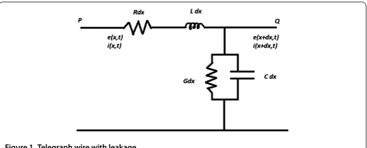
Figure 1 Telegraph wire with leakage.
The challenge is to model an infinite small piece of telegraph wire as an electric circuit since it has a load and a source as indicated by Ohm’s and Kirchhoff ’s laws. The char-acteristics of a small piece of telegraph wire and that of a long transmission line are the same, thus it is sufficient to model an infinite small piece of telegraph wire to represent a transmission line over distance.
Assume that the cable is imperfectly insulated so that there are both capacitance and current leakage to ground as shown in Figure . No two conductors can be perfectly insu-lated due to the current that flows through them as well as the potential difference in the conductors.
Let
x=distance from sending end of the cable,
e(x,t) =potential at any point on the cable at any time,
i(x,t) =current at any point on the cable at any time,
R=resistance of the cable,
L=inductance of the cable,
G=conductance to ground,
C=capacitance to ground.
Voltage drop across the resistor, according to Ohm’s law, is given by
V=I·R. (.)
According to Ohm’s law, voltage drop across the capacitor, where a capacitor gives an integrator circuit, is given by
V=
C
i dt, (.)
and voltage drop across the inductor, where an inductor gives a differentiator circuit, is given by
V=Ldi
The potential atQis equal to the potential atP, minus the drop in potential along the elementPQ. Therefore, if (.)-(.) are combined, it leads to the following equation:
e(x+dx,t) =e(x,t) – (R dx)i–L(dx)∂i ∂t.
Thus
e(x+dx,t) –e(x,t) = –(R dx)i–L(dx)∂i
∂t. (.)
Dividing the above equation bydxand lettingdx→, we get
∂e
∂x= –Ri–L
∂i
∂t. (.)
Likewise, the current atQis equal to the current atP minus the current loss through leakage to ground. Using the equation for current through the capacitor,
i=Cde
dt, (.)
the equation for current now becomes
i(x+dx,t) =i(x,t) – (G dx)i– (C dx)∂e ∂t.
Thus
i(x+dx,t) –i(x,t) = –(G dx)i– (C dx)∂e
∂t. (.)
Dividing the above equation bydxand lettingdx→, we get
∂i
∂x= –Gi–C
∂e
∂t. (.)
If (.) is now differentiated with respect toxand (.) with respect tot, the respective results are
∂e
∂x = –R
∂i
∂x–L
∂i
∂x∂t (.)
and
∂i
∂t∂x= –G
∂e
∂t –C
∂e
∂t. (.)
Using (.) in (.), we get
∂e
∂x = –R
∂i
∂x–L
–G∂e
∂t–C
∂e
∂t
. (.)
Using (.) in (.), we get
∂e
∂x =LC
∂e
∂t + (RC+LG)
∂e
Similarly, we can obtain
Two equations (.) and (.) are known as the telegraphic equations.
Now we apply the proposed method to the following telegraphic equation with the forc-ing functionfto study the stability of the proposed method
ϕtt+ (α+β)ϕt+αβϕ=ϕxx+f(x,t), <x< ,t> , (.)
whereα> ,β≥ are real parameters. Forβ= , equation (.) represents a damped
wave equation. The initial and boundary conditions of type (.) and (.) are prescribed. We denotea=(α+β)
Applying method (.) to differential equation (.) and neglecting local truncation error, we obtain a numerical approximation ofO(k+h) as
The above scheme is conditionally stable (see [, ]).
In order to obtain an unconditionally stable scheme, we may rewrite the above scheme as
The additional terms are of high order and do not affect the accuracy of the scheme. The exact solutionjlsatisfies
Letεlj=jl–ϕjlbe the discretization error at the grid point (xl,tj). Then subtracting (.) from (.), we get the error equation
For stability, we putεlj=ξjeiψlin the homogeneous part of the error equation; we get the
characteristic equation
Using the transformationξ=+–zz, the characteristic equation (.) reduces to
(A–B+C)z+ (A–C)z+ (A+B+C) = . (.)
According to the Routh-Hurwitz criterion, the necessary and sufficient conditions for|ξ|< areA+B+C> ,A–C> ,A–B+C> .
Thus for stability we have the conditions
A+B+C=bcos
Thus the scheme is stable ifη≥ ,γ ≥+λ
λ ,α> ,β≥ for allψ exceptψ= and
π(whenb= ). We treat this case separately.
Forψ= or π(whenb= ), we have the characteristic equation
( +√a)ξ– ξ+ ( –
√
a) = , (.)
whose roots areξ,= , –
√
a
+√a. In this case also|ξ| ≤.
Hence, forα> ,β≥,η≥ ,γ ≥ +λ
λ , scheme (.) is stable for all choices of h> andk> .
Now we consider the fourth-order hyperbolic equation
∂
∂t –
∂
∂x
u=f(x,t), <x< ,t> . (.)
The initial values ofu,ut,utt,utttatt= are known and the boundary values ofu,uxxare known atx= andx= .
Equation (.) in a coupled form can be written as
∂ ∂t –
∂ ∂x
u=v, <x< ,t> , (.a)
∂
∂t –
∂
∂x
v=f(x,t), <x< ,t> . (.b)
Since the grid lines are parallel to coordinate axis, the successive tangential derivatives of
uand its normal derivatives are known on the boundary, that is, the values ofut,utt, . . . are known atx= andx= , and the values ofuxx,uxxt, . . . are known att= . Hence the initial values ofu,ut,v,vtare known att= , and the values ofu,vare known atx= and
x= . Thus, applying scheme (.) to the system of equations (.a) and (.b), we get the following two equations:
Ulj+– Ulj+Ulj–=h
Ujttl++ Ujttl+Ujttl–
–h
Vjl+/+Vˆlj+Vjl–/+Tˆjl, (.a)
Vlj+– Vlj+Vlj–=h
Vjttl++ Vjttl+Vjttl–
–h
flj+/+flj+flj–/+Tˆjl, (.b)
whereUljandVljare the exact solutions of (.a) and (.b), respectively, andTˆjland ˆ
Tjlare ofO(kh+kh+h).
Multiplying throughout byp= (k/h), we may write the above system of equations in
an operator form
+δxδtUlj= pδxUlj+k +δxVlj+pTˆjl, (.a)
Letujlandvjlbe the approximate solutions of (.a) and (.b), respectively, which satisfy
+δxδtujl= pδxujl+k +δxvjl, (.a)
+δxδtvlj= pδxvjl+kflj+/+flj+flj–/. (.b) Let (εu)jl=Ulj–ujland (εv)jl=Vlj–vjlbe the errors at the grid point (xl,tj).
Subtracting (.a) from (.a) and (.b) from (.b), we get the following two error equations:
+δxδt(εu)jl= pδx(εu)jl+k
+δx(εv)jl+pTˆ j
l, (.a)
+δxδt(εv)jl= pδx(εv)jl+pTˆjl. (.b)
Substituting (εv)jl=eiψjeiθlinto the homogeneous part of error equation (.b), we get
sin
ψ
=p
sin(θ
)
–sin(θ
)
. (.)
Since ≤sin(ψ
)≤, from (.), we have
psin
θ
≤ –sin
θ
. (.)
The above inequality holds if
max
psin
θ
≤min
–sin
θ
, (.)
that is, if
<p≤
≈.. (.)
Hence scheme (.b) is stable for <p≤..
Numerically, first we compute (.b) using the value <p≤. and then (.a). Assume that the value of (εv)jlis known in (.a). Then substituting (εu)lj=eiφjeiβlinto
the homogeneous part of (.a), we get
sin
φ
=p
sin(β
)
–sin(β
)
. (.)
Proceeding as above, it is easy to verify that scheme (.a) is also stable for <p≤..
6 Numerical results
exact solution as a test procedure. The linear difference equations have been solved us-ing tridiagonal solver, whereas nonlinear difference equations have been solved usus-ing the Newton-Raphson method. While using the Newton-Raphson method, the iterations were stopped when absolute error tolerance≤–had been achieved. All computations were carried out using MATLAB codes.
The proposed scheme is a three-level scheme. The value ofuatt= is known from the initial condition. To begin the computation, we need the numerical value ofuof required accuracy att=k, so we discuss an explicit method ofO(k) for calculating the value ofuat
first time level in order to solve the differential equation (.) using the proposed scheme (.) which is applicable to problems both in Cartesian and polar coordinates.
Since the values ofu andut are known explicitly att= , so the values of successive tangential derivativesu,ux,uxx, . . . ,utx,utxx, . . . etc. are known att= . An approximation foruatt=kmay be written as
ul =ul +k(ut)l +k
(utt)
l +O
k. (.)
From equation (.), we have
(utt)l =A(x,t,u)uxx+f(x,t,u,ux,ut)l. (.)
Then, using the initial values and their successive tangential derivative values from (.), we obtain the value ofuttatt= , and then subsequently from (.), we can compute the value ofuat first time level, i.e., att=k.
The relation between the exact solutionuexactand the approximate solutionu(h) is given by the following equation:
uexact=u(h) +Mhp+· · ·higher order terms, <x,y< , (.)
wherehis the measure of the mesh discretization,Mis a constant andpis the order (rate) of convergence. If the meshes are to be refined sufficiently, the higher order terms can be neglected. Then the maximum absolute errorsEhcan be approximated as
Eh=Maxuexact–u(h)∼=Mhp. (.)
Taking the logarithm of both sides of (.), we obtain
log(Eh) =log(M) +plog(h). (.)
For two different refined mesh spacinghandh, we have the following two relations:
log(Eh) =log(M) +plog(h), (.a) log(Eh) =log(M) +plog(h), (.b)
whereEh andEh are maximum absolute errors for two uniform mesh sizeshandh,
Table 1 Order of convergence
Problem no. Parameters and time Order
6.1 α0= 12,β0= 8,η=γ= 1,t= 1,σ= 3.2 3.9834
α0=β0=π,η= 0.75,γ= 1.5,t= 1,σ= 3.2 4.0000
α0= 3π,β0=π,η= 2.5,γ= 0.25,t= 1,σ= 3.2 3.9932
6.2 σ= 0.8,ε= 0.01,t= 1 4.0017
σ= 0.8,ε= 0.01,t= 2 4.0017
σ= 0.8,ε= 0.001,t= 1 4.0017
σ= 0.8,ε= 0.001,t= 2 4.0016
6.3 γ= 0.5,t= 1,σ= 3.2 3.9967
γ= 2,t= 1,σ= 3.2 3.9944
6.4 γ= 2,t= 1,σ= 3.2 4.0429
γ= 20,t= 1,σ= 3.2 3.9492
6.5 α= 0.5,t= 1,σ= 1.6 3.9399
α= 0.05,t= 1,σ= 1.6 3.9987
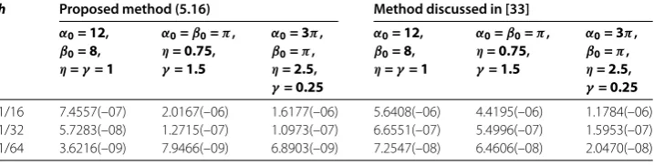
Table 2 Problem 6.1: The maximum absolute errors
h Proposed method (5.16) Method discussed in [33]
α0= 12, β0= 8, η=γ= 1
α0=β0=π, η= 0.75,
γ= 1.5
α0= 3π, β0=π, η= 2.5,
γ= 0.25
α0= 12, β0= 8, η=γ= 1
α0=β0=π, η= 0.75,
γ= 1.5
α0= 3π, β0=π, η= 2.5,
γ= 0.25
1/16 7.4557(–07) 2.0167(–06) 1.6177(–06) 5.6408(–06) 4.4195(–06) 1.1784(–06) 1/32 5.7283(–08) 1.2715(–07) 1.0973(–07) 6.6551(–07) 5.4996(–07) 1.5953(–07) 1/64 3.6216(–09) 7.9466(–09) 6.8903(–09) 7.2547(–08) 6.4606(–08) 2.0470(–08)
h= / for all five problems, for a fixed value ofσ =k/(h), and results are reported
in Table . Assume|E(h)|to be the maximum absolute error foruat a certain time level for a fixed value ofσ=k/(h), then the error behaves like|E(h)| ∼=|Mhp|, implying that
log|E(h)| ∼=log(M) +plog|h|. Thus, on log-log scale the error behaves linearly with a slope that is equal top, the order of convergence.
Problem .(Telegraphic equation)
utt+ (α+β)ut+αβu=uxx+f(x,t), <x< ,t> . (.)
The exact solution is given byu=e–tsinhx. The maximum absolute errors (MAE) are tabulated in Table att= for different values ofα,β,η,γ for a fixed value ofσ= ..
Figures (a) and (b) represent the exact vs numerical solution att= ,σ= .,α= ,
β= ,η= ,γ = ,h= /, and log-log error plot att= ,α=π,β=π,η= .,γ = .,
σ= ., respectively.
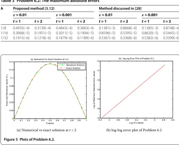
Problem .(Van-der-Pol type nonlinear wave equation)
utt=uxx+εu– ut+f(x,t), <x< ,t> . (.) The exact solution is given by u=e–tsin(πx). The MAE at t= and are tabulated in
(a) Numerical vs exact solution att= (b) log-log error plot of Problem .
Figure 2 Plots of Problem 6.1.
Table 3 Problem 6.2: The maximum absolute errors
h Proposed method (3.12) Method discussed in [28]
ε= 0.01 ε= 0.001 ε= 0.01 ε= 0.001
t = 1 t = 2 t = 1 t = 2 t = 1 t = 2 t = 1 t = 2
1/8 0.4935(–4) 0.3139(–4) 0.4843(–4) 0.3063(–4) 0.1381(–3) 0.8668(–4) 0.1385(–3) 0.8748(–4) 1/16 0.3068(–5) 0.1951(–5) 0.3011(–5) 0.1904(–5) 0.8596(–5) 0.5395(–5) 0.8620(–5) 0.5445(–5) 1/32 0.1915(–6) 0.1218(–6) 0.1879(–6) 0.1189(–6) 0.5367(–6) 0.3368(–6) 0.5382(–6) 0.3399(–6)
(a) Numerical vs exact solution att= (b) log-log error plot of Problem .
Figure 3 Plots of Problem 6.2.
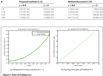
Problem .(Nonlinear wave equation)
utt=uxx+γu(ux+ut) +f(x,t), <x< ,t> . (.)
The exact solution is given byu=e–tcoshx. The MAE are tabulated in Table att=
Table 4 Problem 6.3: The maximum absolute errors
h Proposed method (3.12) Method discussed in [35]
γ= 0.5 γ= 2 γ= 0.5 γ= 2
1/8 5.0419(–04) 9.3631(–04) 2.1822(–03) 1.5863(–03)
1/16 3.1579(–05) 5.8584(–05) 1.6354(–04) 1.1132(–04)
1/32 1.9734(–06) 3.6602(–06) 1.1177(–05) 7.6658(–06)
1/64 1.2362(–07) 2.2966(–07) 8.6172(–07) 5.8284(–07)
(a) Numerical vs exact solution att= (b) log-log error plot of Problem .
Figure 4 Plots of Problem 6.3.
Table 5 Problem 6.4: The maximum absolute errors
h Proposed method (3.12) Method discussed in [35]
γ= 2 γ= 20 γ= 2 γ= 20
1/8 2.2955(–04) 1.8526(–03) 7.4446(–04) 5.2318(–03)
1/16 1.3364(–05) 1.0955(–04) 5.7172(–05) 3.3478(–04)
1/32 8.2180(–07) 6.9282(–06) 3.6105(–06) 2.1633(–05)
1/64 4.9859(–08) 4.4854(–07) 2.3129(–07) 1.4261(–06)
Problem .(Quasi-linear equation)
utt=
+uuxx+γuux+f(x,t), <x< ,t> . (.)
The exact solution is given byu=e–tsin(πx). The MAE are tabulated in Table att=
forγ = and for a fixed value ofσ= .. Figures (a) and (b) represent the exact vs numerical solution att= ,γ = ,h= / and log-log error plot att= ,γ = , respec-tively.
Problem .(Fourth-order nonlinear hyperbolic equation)
∂
∂t –
∂
∂x
u=αuux+f(x,t), <x< ,t> . (.)
(a) Numerical vs exact solution att= (b) log-log error plot of Problem .
Figure 5 Plots of Problem 6.4.
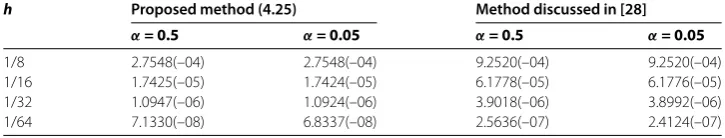
Table 6 Problem 6.5: The maximum absolute errors
h Proposed method (4.25) Method discussed in [28]
α= 0.5 α= 0.05 α= 0.5 α= 0.05
1/8 2.7548(–04) 2.7548(–04) 9.2520(–04) 9.2520(–04)
1/16 1.7425(–05) 1.7424(–05) 6.1778(–05) 6.1776(–05)
1/32 1.0947(–06) 1.0924(–06) 3.9018(–06) 3.8992(–06)
1/64 7.1330(–08) 6.8337(–08) 2.5636(–07) 2.4124(–07)
In order to solve (.), we put
∂
∂t –
∂
∂x
u=v. (.)
Hence (.) reduces to a system of coupled nonlinear equations of the form
∂ ∂t –
∂ ∂x
u=v, <x< ,t> , (.)
∂ ∂t –
∂ ∂x
v=αuux+f(x,t), <x< ,t> . (.)
Since the grid lines are parallel to coordinate axis, successive tangential derivatives ofu
and its normal derivatives are known on the boundary. Hence the initial values ofu,ut,v,
vt are known att= , and the values ofu,vare known atx= andx= . Thus applying scheme (.), we can solve the system of equations (.) and (.).
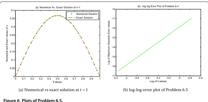
The exact solution isu=e–tsin(πx). The maximum absolute errors foruare tabulated
in Table att= forα= . and . for a fixed value ofσ= .. Figures (a) and (b) represent the exact vs numerical solution att= ,α= .,h= / and log-log error plot att= ,α= ., respectively.
7 Concluding remarks
(a) Numerical vs exact solution att= (b) log-log error plot of Problem .
Figure 6 Plots of Problem 6.5.
compression function in derivation of the method. For a fixed parameterσ =k/h, the proposed method behaves like a fourth-order method. The accuracy and efficiency of the proposed method are exhibited from the numerical computations. The proposed method for scalar equation has been extended in a vector form to solve the system of quasi-linear hyperbolic pdes. For the telegraphic equation, the method is shown to be uncondition-ally stable, and the stability condition for solving a fourth-order linear hyperbolic pde has also been established. The method is directly applicable to quasilinear hyperbolic pdes irrespective of the coordinate system, which brings an edge over other existing methods.
Competing interests
The authors declare that they have no competing interests.
Authors’ contributions
RKM derived the method for scalar quasilinear hyperbolic equation and discussed the stability analysis. GK extended the method to solve the system of nonlinear hyperbolic equations and carried out all the computational work. All the authors read and approved the final manuscript.
Author details
1Department of Applied Mathematics, South Asian University, Akbar Bhawan, Chanakyapuri, New Delhi, 110021, India. 2Permanent address: Department of Mathematics, I.P. College for Women, University of Delhi, Delhi, 110054, India.
Acknowledgements
This work is supported by I.P. College for Women, University of Delhi. The authors thank the reviewers for their valuable suggestions, which substantially improved the standard of the paper.
Publisher’s Note
Springer Nature remains neutral with regard to jurisdictional claims in published maps and institutional affiliations.
Received: 23 January 2017 Accepted: 21 March 2017 References
1. Li, WD, Zhao, L: An analysis for a high order difference scheme for numerical solution toutt=A(x,t)uxx+f(x,t,u,ux,ut). Numer. Methods Partial Differ. Equ.23, 484-498 (2007)
2. Bickley, WG: Piecewise cubic interpolation and two-point boundary value problems. Comput. J.11, 206-208 (1968) 3. Fyfe, DJ: The use of cubic splines in the solution of two-point boundary value problems. Comput. J.12, 188-192
(1969)
4. Papamichael, N, Whiteman, JR: A cubic spline technique for the one-dimensional heat conduction equation. J. Inst. Math. Appl.11, 111-113 (1973)
5. Raggett, GF, Wilson, PD: A fully implicit finite difference approximation to the one-dimensional wave equation using a cubic spline technique. J. Inst. Math. Appl.14, 75-77 (1974)
7. Jain, MK, Aziz, T: Spline function approximation for differential equation. Comput. Methods Appl. Mech. Eng.26, 129-143 (1981)
8. Jain, MK, Aziz, T: Cubic spline solution of two-point boundary value problems with significant first derivatives. Comput. Methods Appl. Mech. Eng.39, 83-91 (1983)
9. Jain, MK, Iyengar, SRK, Pillai, ACR: Difference schemes based on splines in compression for the solution of conservation laws. Comput. Methods Appl. Mech. Eng.38, 137-151 (1983)
10. Kadalbajoo, MK, Patidar, KC: Numerical solution of singularly perturbed two point boundary value problems by spline in compression. Int. J. Comput. Math.77, 263-284 (2001)
11. Kadalbajoo, MK, Patidar, KC: Numerical solution of singularly perturbed two-point boundary value problems by spline in tension. Appl. Math. Comput.131, 299-320 (2002)
12. Khan, A, Aziz, T: Parametric cubic spline approach to the solution of a system of second order boundary value problems. J. Optim. Theory Appl.118, 45-54 (2003)
13. Kadalbajoo, MK, Aggarwal, VK: Cubic spline for solving singular two-point boundary value problems. Appl. Math. Comput.156, 249-259 (2004)
14. Mohanty, RK, Jha, N, Evans, DJ: Spline in compression method for the numerical solution of singularly perturbed two point singular boundary value problems. Int. J. Comput. Math.81, 615-627 (2004)
15. Mohanty, RK, Evans, DJ, Arora, U: Convergence spline in tension methods for singularly perturbed two point singular boundary value problems. Int. J. Comput. Math.82, 55-66 (2005)
16. Mohanty, RK, Jha, N: A class of variable mesh spline in compression methods for singularly perturbed two point single boundary value problems. Appl. Math. Comput.168, 704-716 (2005)
17. Mohanty, RK, Arora, U: A family of non-uniform mesh tension spline methods for singularly perturbed two-point singular boundary value problems with significant first derivatives. Appl. Math. Comput.172, 531-544 (2006) 18. Rashidinia, J, Jalilian, R, Kazemi, V: Spline methods for the solutions of hyperbolic equations. Appl. Math. Comput.190,
882-886 (2007)
19. Rashidinia, J, Mohammadi, R: Non polynomial cubic spline methods for the solution of parabolic equations. Int. J. Comput. Math.85, 843-850 (2008)
20. Siraj-ul-Islam, Tirmizi, SIA: Nonpolynomial spline approach to the solution of a system of second order boundary value problems. Appl. Math. Comput.173, 1208-1218 (2006)
21. Siraj-ul-Islam, Tirmizi, SIA, Asharaf, S: A class of methods based on nonpolynomial spline functions for the solution of special fourth order boundary value problems with engineering applications. Appl. Math. Comput.174, 1169-1180 (2006)
22. Ding, H, Zhang, Y: Parametric spline methods for the solution of hyperbolic equations. Appl. Math. Comput.204, 938-941 (2008)
23. Mohanty, RK, Jain, MK: High accuracy cubic spline alternating group explicit methods for 1D quasilinear parabolic equations. Int. J. Comput. Math.86, 1556-1571 (2009)
24. Mohanty, RK, Gopal, V: A fourth-order finite difference method based on spline in tension approximation for the solution of one-space dimensional second-order quasilinear hyperbolic equations. Adv. Differ. Equ.2013, Article ID 70 (2013)
25. Mohanty, RK, Jha, N, Kumar, R: A new variable mesh method based on non-polynomial spline in compression approximations for 1D quasilinear hyperbolic equations. Adv. Differ. Equ.2015, Article ID 337 (2015)
26. Mohanty, RK, Singh, S: High accuracy Numerov type discretization for the solution of one dimensional non-linear wave equation with variable coefficients. J. Adv. Res. Sci. Comput.3(1), 53-66 (2011)
27. Mohanty, RK, Gopal, V: An off-step discretization for the solution of 1-D mildly non-linear wave equations with variable coefficients. J. Adv. Res. Sci. Comput.4(2), 1-13 (2012)
28. Mohanty, RK, Jain, MK, George, K: On the use of high order difference methods for the system of one space second order non-linear hyperbolic equations with variable coefficients. J. Comput. Appl. Math.72, 421-431 (1996) 29. Mohanty, RK, Arora, U: A new discretization method of order four for the numerical solution of one space
dimensional second order quasi-linear hyperbolic equation. Int. J. Math. Educ. Sci. Technol.33, 829-838 (2002) 30. Mohanty, RK, Gopal, V: High accuracy cubic spline difference approximation for the solution of one-space
dimensional non-linear wave equations. Appl. Math. Comput.218, 4234-4244 (2011)
31. Gopal, V, Mohanty, RK, Jha, N: New nonpolynomial spline in compression method ofO(k2+h4) for the solution of 1D wave equation in polar coordinates. Adv. Numer. Anal.2013, Article ID 470480 (2013)
32. Mohanty, RK: Stability interval for explicit difference schemes for multi-dimensional second order hyperbolic equations with significant first order space derivative terms. Appl. Math. Comput.190, 1683-1690 (2007) 33. Mohanty, RK: An unconditionally stable difference scheme for the one-space-dimensional linear hyperbolic
equation. Appl. Math. Lett.17, 101-105 (2004)
34. Mohanty, RK: New unconditionally stable difference schemes for the solution of multi-dimensional telegraph equations. Int. J. Comput. Math.86, 2061-2071 (2009)
35. Mohanty, RK, Gopal, V: High accuracy non-polynomial spline in compression method for one-space dimensional quasi-linear hyperbolic equations with significant first order space derivative term. Appl. Math. Comput.238, 250-265 (2014)
36. Mohanty, RK, Khurana, G: A new fast numerical method based on off-step discretization for two-dimensional quasilinear hyperbolic partial differential equations. Int. J. Comput. Methods (2016). doi:10.1142/S0219876217500311 37. Mohanty, RK, Setia, N: A new high accuracy two-level implicit off-step discretization for the system of two space
dimensional quasi-linear parabolic partial differential equations. Appl. Math. Comput.219, 2680-2697 (2012) 38. Mohanty, RK, Jain, MK, Dhall, D: High accuracy cubic spline approximation for two dimensional quasi-linear elliptic
boundary value problems. Appl. Math. Model.37, 155-171 (2013)
39. Mohanty, RK, Gopal, V: A new off-step high order approximation for the solution of three-space dimensional nonlinear wave equations. Appl. Math. Model.37, 2802-2815 (2013)
40. Mohanty, RK, Setia, N: A new high order compact off-step discretization for the system of 3D quasi-linear elliptic partial differential equations. Appl. Math. Model.37, 6870-6883 (2013)
42. Mohanty, RK, Singh, S, Singh, S: A new high order space derivative discretization for 3D quasi-linear hyperbolic partial differential equations. Appl. Math. Comput.232, 529-541 (2014)
43. Mohanty, RK, Kumar, R: A new fast algorithm based on half-step discretization for one space dimensional quasi-linear hyperbolic equations. Appl. Math. Comput.244, 624-641 (2014)
44. Mohanty, RK, Kumar, R: A novel numerical algorithm of Numerov type for 2D quasi-linear elliptic boundary value problems. Int. J. Comput. Methods Eng. Sci. Mech.15, 473-489 (2014)
45. Mohanty, RK, Setia, N: A new high accuracy two-level implicit off-step discretization for the system of three space dimensional quasi-linear parabolic partial differential equations. Comput. Math. Appl.69, 1096-1113 (2015) 46. Varga, RS: Matrix Iterative Analysis, 2nd edn. Springer, Berlin (2000)
47. Hageman, LA, Young, DM: Applied Iterative Methods. Dover, New York (2004)