R E S E A R C H
Open Access
Jacobi spectral solution for weakly singular
integral algebraic equations of index-1
Jingjun Zhao
*and Shiying Wang
*Correspondence: [email protected]
Department of Mathematics, Harbin Institute of Technology, Harbin, 150001, China
Abstract
This paper is concerned with obtaining the approximate solution of a class of semi-explicit Integral Algebraic equations (IAEs) of index-1 with weakly singular kernels. Some function transformations and variable transformations are used to change the equations into integral equations defined on the standard interval [–1, 1], so that the solution of the new system possesses better regularity and the Jacobi orthogonal polynomial theory can be applied conveniently. A Jacobi collocation method is proposed and its convergence analysis is provided, which theoretically justifies the spectral rate of convergence. The numerical results are given to verify our theoretical analysis.
MSC: 65R20
Keywords: integral algebraic equations; Jacobi collocation method; system of weakly singular Volterra equations; index of IAEs; error analysis
1 Introduction
In this paper, we consider the following system of Volterra Integral equations (VIEs) with weakly singular kernels:
⎧ ⎪ ⎪ ⎪ ⎨ ⎪ ⎪ ⎪ ⎩
y(t) =f(t) +
t
(t–s)–
αK
(t,s)y(s)ds
+t(t–s)–αK
(t,s)z(s)ds,
=f(t) +
t
(t–s) –αK
(t,s)y(s)ds
+t(t–s)–αK
(t,s)z(s)ds,
t∈I= [,T], (.)
where <α=pq < (p,q∈N,p<q), the functionsf,fandKij(·,·) (i,j= , ) are known
to be smooth onIandD={(t,s) : ≤s≤t≤T}, respectively, andy(t),z(t) are unknown solutions. We assume thatf() = ,|k(t,t)| ≥k> ,∀t∈I. Under these conditions,
system (.) is called a system of Weakly Singular Integral Algebraic equations (WSIAEs) of index . System (.) can be written in the following form:
A(t)X(t) =F(t) + t
(t–s)–αK(t,s)X(s)ds,
where
A=
, X(t) =
y(t),z(t)T, F(t) =f(t),f(t)
T
,
K(t,s) =
K(t,s) K(t,s)
K(t,s) K(t,s)
.
In practical applications, one frequently encounters system (.). A good source on ap-plications of IAEs with weakly singular kernels is the initial (boundary) value problems for the semi-infinite strip and temperature boundary specification including two/three-phase inverse Stefan problems [–]. A wide ranging description of IAEs arising in applications is given in []. Several numerical methods for integral algebraic equations have been pro-posed (see e.g.[–]). However, as far as we know the numerical analysis of WSIAEs is largely incomplete and this is a new topic for research. The existence and uniqueness for the solution of WSIAEs has been given in [, ]. The piecewise polynomial colloca-tion method for system (.) and the concept of tractability index have been considered by Brunner []; he analyzed the regularity of the solutions using conditions that hold for the first and second kind Volterra integral equations. Recently, the effective numerical method based on the Chebyshev collocation scheme is designed for system (.) in [] and its convergence analysis is provided.
The solutions of system (.) usually have a weak singularity att= , whose derivatives are unbounded at t= . To overcome this difficulty, we use the idea of the authors in []. Both function transformation and variable transformation are used to change the system into a new system defined on the standard interval [–, ], so that the solutions of the new system possess better regularity and the Jacobi spectral collocation method can be applied conveniently. The aim of this work is to use the Jacobi collocation method to numerically solve the WSIAEs (.) and then a rigorous error analysis is provided in the weightedL-norm which shows the spectral rate of convergence is attained.
This paper is organized as follows. Some useful results for establishing the convergence results will be provided in Section . In Section , we carry out the Jacobi collocation approach for system (.). The convergence of the method in the weightedL-norm as a
main result of the paper is given in Section . Section gives some numerical experiments. The final section contains conclusions and remarks.
2 Some useful results
In this section, we discuss how the weakly singular IAEs can be changed to treat the prob-lem. Furthermore, the index concept for WSIAEs which plays a fundamental role in both the analysis and the development of numerical algorithms for IAEs is discussed.
2.1 Index definitions for WSIAEs
There are several definitions of index in literature, not all completely equivalent, such as the tractability index (see,e.g.Definition (..) from []), the left index [] and differen-tiation index []. Generally, the difficulties are arising in the theoretical and numerical analysis of IAEs relevant to the index notion.
In this paper, we use the concept of the differentiation index which measures how far the main WSIAE is apart from a regular system of VIEs. Namely, the number of analytical differentiations of system (.) until it can be formulated as a regular system of Volterra integral equations is called the differentiation index.
of the second equation of (.) by the factor (u–t)α–and integrate with respect to t,
the following first kind Volterra integral equation with regular bounded kernels will be obtained:
= t
H(t,s)y(s)ds+
t
H(t,s)z(s)ds+Gα(f), (.)
where
H(t,s) =
K(s+ (t–s)υ,s)
υα( –υ)–α dυ, H(t,s) =
K(s+ (t–s)υ,s)
υα( –υ)–α dυ,
and
Gα(f) =
t
(t–s)α–f (s)ds.
We get the following second kind integral equation by differentiation of equation (.):
=H(t,t)y(t) +H(t,t)z(t) +
t
∂H(t,s)
∂t y(s)ds
+ t
∂H(t,s)
∂t z(s)ds+G
α(f), (.)
whereHj(t,t) =sin(παπ)Kj(t,t) (j= , ) andGα(f) =
t
(t–s)
α–f
(s)ds. In fact,Gα(f) can
be obtained using integration by parts toGα(f) withf() = .
Because|K(t,t)| ≥k> , we have|H(t,t)|> , then equation (.) together with the
first equation of (.) is a system of regular Volterra integral equation.
But it should be noted that this reduction (differentiation) is not useful from a numer-ical point of view and such a definition may be useful for understanding the underlying mathematical structure of a WSIAEs, and hence choosing a suitable numerical method for their solutions.
2.2 Smoothness of the solution
We assume that the Hölder spaceC,β([,T]) =Cβ([,T]) is defined to be a subspace of C([,T]) that consists of functions which are Hölder continuous with the exponentβ. For m∈Z+andβ∈(, ], we similarly define the Hölder space
Cm,β[,T]=f ∈Cm[,T]|Dυf ∈C,β[,T],∀υ,|υ|=m. It is shown in [] that this is a Banach space with the following norm:
fCk,β([,T])=fCm([,T])+
|υ|=m
sup
|Dυf(x) –Dυf(y)| |x–y|β
x,y∈[,T],x=y
.
smooth solutions. Using the idea of Li and Tang in [], one can overcome this difficulty by introducing the following variable transformation:
t=uq, u=√qt, s=wq, w=√q
s, (.)
to change (.) to the following system:
⎧
The existence and uniqueness results and the smoothness behavior of solutionsyˆandzˆ of system (.) can be obtained from the corresponding discussions of the classical the-ory of Volterra integral equations with weakly singular kernels from [] (seee.g. Theo-rems .. and .. for further details).
3 The Jacobi collocation method
We first introduce some notations. Letωα,β(x) = ( –x)α( +x)β (α,β > –) be a weight function in the usual sense. As defined in [], let us denoteJnα,β(x) the Jacobi polynomial of
degreenwith respect to weightωα,β(x). It is well known that the set of Jacobi polynomials
{Jnα,β(x)}∞n=forms a completeLωα,β(–, ) orthogonal system, whereLωα,β(–, ) is the space
Particularly, whenα=β= , the Jacobi polynomials become Legendre polynomials, and whenα=β= –, the Jacobi polynomials become Chebyshev polynomials.
For the sake of obtaining a Jacobi spectral method for system (.), we employ the linear transformation
to rewrite system (.) as follows:
wheref˜(v) =fˆ(
It is well known that, in the Jacobi collocation method, we usey˜Nand˜zNof the following
form:
to approximate the solutionsy˜andz˜, wherevkare the Gauss-Jacobi quadrature points and
Lkare the interpolating Lagrange polynomials
Lk(v) =
can be approximated by a univariate Lagrange interpolating polynomial as follows:
IN
Substituting equations (.) and (.) into (.) and inserting the collocation pointsvk
(k= , , . . . ,N) in the obtained equation, one obtains the following system of linear
equa-by solving the linear system (.) and finally the approximate solutions˜yN andz˜N will be
computed by substituting these coefficients into (.).
4 Error estimate
To prove the error estimate in the weighted L-norm, we first introduce some lemmas
Lemma ([]) Let IN be a linear operator from Ck,β([–, ])to PN,then∀k∈N, β ∈
[, ],there exists a positive constant Ck,β,such that∀f ∈Ck,β([–, ]),∃INf∈PN,s.t.,f–
INfL∞≤Ck,βN–(k+β)fCk,β([–,]).
Lemma ([]) Let{Lj(x)}Nj=be Lagrange interpolation polynomials with the Jacobi Gauss
points{xj}Nj=,then
INL∞= max x∈(–,)
N
i=
Li(x)=
O(logN), – <α,β≤–, O(N+γ), otherwise,
γ =max{α,β}.
Lete(v) =y˜N(v) –y˜(v),e(v) =z˜N(v) –z˜(v) denote the error functions. The following
main theorem reveals the convergence results of the presented scheme in the weighted L-norm.
Theorem Consider the index-weakly singular integral algebraic equations(.)and its
transformed representation(.).LetD˜ ={(t,s) : –≤x≤v≤T}, (˜yN,˜zN)be the
approxi-mated solution for the exact solution(y˜,z˜)of(.)based on the spectral collocation scheme (.)and suppose the following conditions hold:
() K˜j∈Cm(D˜)(j= , ),f˜∈Cm[–, ];
() K˜j∈Cm+(D˜)(j= , ),f˜∈Cm+[–, ]withf˜(–) = ; () K˜(v,v)> ,∀v∈[–, ].
Then for sufficiently large N,
eL
ωα,β(–,)
=˜yN–y˜L
ωα,β(–,)≤
O(N–mlogN), – <α,β≤– ,
O(N+γ–mlogN), otherwise,
eL
ωα,β(–,)
=˜zN–˜zL
ωα,β(–,)≤
O(N–mlogN), – <α,β≤– ,
O(N+γ–mlogN), otherwise,
whereγ =max{α,β}.
Proof First, the first equation of system (.) can be rewritten as
˜
y(vk) =f˜(vk) + N
n=
N
l=
(anl+bnl)Wnl(vk), (.)
where
anl=
˜
yn(K˜)n, n=l,
˜
yn(K˜)l+y˜l(K˜)n, n=l,
bnl=
˜
zn(K˜)n, n=l,
˜
zn(K˜)l+˜zl(K˜)n, n=l,
and
(K˜ij)n=K˜ij(vk,vn) (i,j= , ), ˜yn=y˜(vn),
Wnl(vk) =
vk
–
Using these notations, equation (.) can be written as
and subtracting equation (.) from the first equation of (.), we have
e(v) =IN
Equation (.) can be rewritten as follows:
W=IN
Next, by using the second equation of (.), we have
IN
For the second equation of (.), using a similar procedure as outlined for obtaining the relation (.), and then inserting equation (.) into the resulting equation, we get
=
Using a similar method for obtaining equation (.) in Section , equation (.) can be written as
Now, we rewrite equation (.) as
–H˜(v,v)e(v) –H˜(v,v)e(v)
= v
–
(v–x)–α
(v–x)α∂H˜(v,v) ∂v e(x)
dx
+ v
–
(v–x)–α
(v–x)α∂H˜(v,v) ∂v e(x)
dx+Gα(F), (.)
equations (.) and (.) can be written in the form of the compact matrix representation:
H(v,v)E(v) = v
–
(v–x)–αR(v,x)E(x)dx+M, (.)
where
H(v,v) =
–H˜(v,v) –H˜(v,v)
, R(v,x) =
˜
K(v,x) K˜(v,x)
(v–x)α ∂K˜(v,x)
∂v (v–x)
α ∂K˜(v,x)
∂v
,
E(v) =
e(v)
e(v)
, M=
W+W+W+W+W+IN(Z(v)) +IN(Z(v))
Gα(F) .
From equation (.),H˜(v,v) =sinπαπK˜(v,v) andH˜(v,v) = sinαπ
π K˜(v,v), and from the condition () of Theorem ,| ˜K(v,v)|> ,∀v∈[–, ], so the matrixH(v,v) is invertible
and its inverse can be written as
H–(v,v) =
–K˜(v,v) ˜
K(v,v)
–π sin(απ)K˜(v,v)
.
Multiplying equation (.) byH–(v,v) yields
E(v)L
ω(–,)≤
v
–
(v–x)–αE(v)L
ω(–,)dx+ ˆNLω(–,), (.)
where =max–≤x<v≤H–(v,v)R(v,x)
Lω(–,)andNˆ =H
–(v,v)M.
By the generalized Gronwall inequality [, Lemma (.)], one obtains
E(v)L
ω(–,)≤
v
–
(v–x)–α ˆNL
ω(–,)dx+ ˆNLω(–,). (.)
It follows from the generalized Hardy inequality [, Lemma ] that
E(v)L
ω(–,)≤C ˆNLω(–,). (.)
From now on, for simplicity, we denote · L
ω(–,)by · and try to derive the error
bounds for the proposed method step by step.
Step : We now estimate the error bounds for Wi (i= , . . . , ). SinceIN denotes the
interpolation operator, we have
It is noted that
W=INe–e=INe–IN
IN(e)
+IN(e) –e ≤ INe–IN(e)+IN(e) –e
≤INL∞+ e–IN(e)L∞,
whereIN is defined in Lemma , and
e=
v
–
(v–x)–αK˜(v,x)e(x)dx. (.)
Using Lemma fork= , Lemma , and Lemma (.) from [], we obtain
W ≤
C(logN+ )N–βe
C,β([–,])≤ClogNN–βeL∞, – <α,β≤ ,
C(N+γ+ )N–βe
C,β([–,])≤CN
+γN–βeL∞, otherwise. Then using the inequality (..) from [], we have
W ≤
ClogNN–m–β|˜y|
Hωm,N(–,), – <α,β≤ ,
CN+γ–β–m|˜y|
Hωm,N(–,), otherwise.
(.)
Here
|˜y|Hm,N
ω (–,)=
m
j=min(m,N+)
y˜(j)L
ω(–,)
. (.)
Similarly,
W ≤
ClogNN–m–β|˜z|
Hmω,N(–,), – <α,β≤/,
CN+γ–β–m|˜z|
Hmω,N(–,), otherwise, W ≤
ClogNN–β˜y
L∞, – <α,β≤/,
CN+γ–β˜yL∞, otherwise,
W ≤
ClogNN–β˜z
L∞, – <α,β≤/,
CN+γ–β˜zL∞, otherwise,
W ≤CN–m|˜f|Hm,N
ω (–,).
Step : In this step, we estimateIN(Z(v)) andIN(Z(v)). Using Lemma , we have
IN
Z(v)≤ max ≤k≤N
Z(vk)INL∞
≤ max
≤k≤N
Z(vk)·
O(logN), – <α,β≤–,
Furthermore, from (.) we obtain
Z(vk)=
–vk(vk–x)–α
IN
˜ K(vk,x)
–K˜(vk,x)y˜N(x)
dx
≤CIN
˜ K(vk,x)
–K˜(vk,x)L∞˜yNL∞
vk
–
(vk–x)–αdx.
Using the transformation (.), we have vk
–
(vk–x)–αdx= (vk+ )(–α)B(, –α),
whereB(·,·) denotes the Euler Beta function. Then using the inequality (..) from [], we have
Z(vk)≤C(vk+ )(–α)B(, –α)N
–mK˜
(vk,x)Hm,N
ω (–,)˜yNL∞. (.)
From (.), we obtain
IN
Z(v)≤
ClogNN–m ˜yNL∞, CN+γ–m
˜yNL∞,
(.)
where
ij=B(, –α) max
≤k≤N(vk+ )
(–α)K˜
ij(vk,x)Hm,N
ω (–,) (i,j= , ).
Similarly, we have
IN
Z(v)≤
ClogNN–m ˜yNL∞, CN+γ–m
˜yNL∞.
Step : Here, our aim is to find a bound forGα(F) using the suitable inequalities as well as the previously obtained bounds. Therefore, we estimate equation (.) as
Gα(F)≤ v
–
(v–x)α–F(x)dx.
By using the generalized Hardy inequality from [], it can be seen that
Gα(F)≤CF(x)≤CW+W+IN
Z(v)+IN
Z(v). (.)
Using the inequality (..) from [], we have
W≤CN–m| ˜e|Hm,N
ω (–,),
wheree=
v
–(v–x)–
αK˜
(v,x)e(x)dx.
Letm= in (.), we have
W≤C∂e ∂v
Moreover, using integration by parts and the generalized Hardy inequality, we have
∂e
∂v
≤Ce+e.
Now, using the inequalities (..) and (..) from [] yields
W≤CN–m+N–m|˜y|Hm,N
ω (–,).
Similarly,
W≤CN–m+N–m|˜z|Hm,N
ω (–,).
On the other hand, using the inequality (..) from [] and equation (.), we obtain
INZ(v)≤CNIN
Z(v)≤
ClogNN–m ˜yNL∞, CN+γ–m
˜yNL∞.
Also we have
INZ(v)≤CNIN
Z(v)≤
ClogNN–m ˜yNL∞, CN+γ–m
˜yNL∞.
Finally, the above estimates together with equation (.) lead to Theorem .
It is noted in [] that the function transformation generally makes the resulting equa-tions and approximaequa-tions more complicated. As discussed in [, p.], we can also obtain the error estimates for the numerical solutions to the WSIAEs (.).
Theorem Consider the index-WSIAEs(.).Let(yN,zN)be the spectral collocation
ap-proximation for the exact solution(y,z)of system(.),and suppose the following conditions hold:
() Kj∈Cm(D)(j= , ),f∈Cm(I);
() Kj∈Cm+(D)(j= , ),f∈Cm+(I)withf() = ; () |K(v,v)|> ,∀v∈I.
Then for sufficiently large N,
yN–y ≤
O(N–mlogN), – <α,β≤– ,
O(N+γ–mlogN), otherwise,
zN–z ≤
O(N–mlogN), – <α,β≤– ,
O(N+γ–mlogN), otherwise,
whereγ =max{α,β}.
5 Numerical experiments
the approximate solution for coupled system of weakly singular integral algebraic equa-tions which consist of both the first and the second kind Volterra integral equaequa-tions. To our knowledge, there are no other results as regards the numerical analysis of WSIAEs except [], which designed an effective numerical method based on the Chebyshev col-location scheme for system (.) and provided its convergence analysis. It is noted that the Jacobi collocation method becomes the Chebyshev collocation method forα=β= –/. In this section, some numerical examples are given to show the validity of the proposed method. Variable transformations (.) and linear transformations (.) are used to change the WSIAEs system into a new system such that its solutions have better regularity. All the computations were performed using the softwareMatlab®. These problems are solved us-ing the Jacobi collocation method forα=,β=. In order to show the behavior of the errors, we define the weightedL-norm by
eL
ωα,β(–,)
=
–
|e|ωα,β(t)dt
,
whereωα,β(x) = ( –x)α( +x)β(α,β> –) is the Jacobi weight function.
Example Consider the following index- WSIAEs system:
AX(t) =G(t) + t
(t–s)–K(t,s)X(s)ds, t∈[, ],
where
A=
, K(t,s) =
t+ t+s
s+ t+s+ ,
X(t) =y(t),z(t)T, F(t) =f(t),f(t)
T
,
andf,fare chosen such that the exact solution is
y(t) =arctan√t, z(t) =e
t–
√
t .
Becausey(t) =(+t– t),z(t) =t–(et–
t +et), it is noted thaty∼t–
andz∼t– att→.
Forα=pq =, by using variable transformation t=u, the smooth solutions yˆ=y(u),
ˆ
z=z(u) are obtained. Insertingyˆ,zˆin the WSIAEs and using the transformation (.), we
have
AX˜(v) =F˜(v) + t
(v–x)–K˜(v,x)X˜(x)dx, v∈[–, ], (.)
where
˜
K(v,x) =
˜
K(v,x) K˜(v,x) ˜
K(v,x) K˜(v,x)
, X˜(v) =y˜(v),˜z(v)T, F˜(v) =f˜(v),f˜(v)
T
Table 1 L2
ωα,β(–1, 1) errors for Example 1
N y˜N–y˜L2
ωα,β(–1,1) ˜
zN–z˜L2
ωα,β(–1,1)
4 1.75×10⁻⁴ 1.61×10⁻³ 5 3.34×10⁻⁵ 2.59×10⁻⁴ 6 7.33×10⁻⁶ 5.80×10⁻⁵ 7 4.12×10⁻⁷ 5.62×10⁻⁶ 8 2.35×10⁻⁷ 6.15×10⁻⁶ 9 4.65×10⁻⁸ 3.96×10⁻⁷
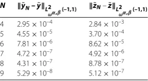
Table 2 L2
ωα,β(–1, 1) errors for Example 2
N y˜N–y˜L2
ωα,β(–1,1)
˜zN–z˜L2
ωα,β(–1,1)
4 2.95×10⁻⁴ 2.84×10⁻³ 5 4.55×10⁻⁵ 3.70×10⁻⁴ 6 7.81×10⁻⁶ 8.62×10⁻⁵ 7 4.72×10⁻⁷ 4.92×10⁻⁶ 8 4.31×10⁻⁷ 8.78×10⁻⁷ 9 5.29×10⁻⁸ 5.12×10⁻⁷
Let (˜yN,˜zN) denote the approximation of the exact solution (˜y,˜z) that is given by equation
(.). The proposed Jacobi collocation methods are applied for system (.). Table shows the errors for (y˜,z˜). It is seen that the desired exponential rate of convergence is obtained.
Example
AX(t) =G(t) + t
(t–s)–K(t,s)X(s)ds, t∈[, ],
where
A=
, K(t,s) =
e√s+t(t+s+ ) coss(t+s)
e√s+t+(t+s) sin(s+ )(ts+ ) ,
X(t) =y(t),z(t)T, G(t) =f(t),f(t)
T
,
andf,fare chosen such that the exact solution is
y(t) =exp(√t), z(t) =sin√t.
In Table we present the weightedL-norm of errors for the numerical solutions by
using the spectral collocation method.
6 Conclusions
the method in the weighted L-norm was obtained. Numerical results are presented to
confirm the theoretical prediction of the exponential rate of convergence.
Competing interests
The authors declare that they have no competing interests.
Authors’ contributions
All authors contributed equally to the writing of this paper. All authors read and approved the final manuscript.
Acknowledgements
The authors would like to acknowledge the anonymous referees for their careful reading of the manuscript and constructive comments. This work is supported by the National Natural Science Foundation of China (11101109, 11271102), Natural Science Foundation of Hei-long-jiang Province of China (A201107) and SRF for ROCS, SEM.
Received: 21 January 2014 Accepted: 28 May 2014 Published:05 Jun 2014
References
1. Cannon, JR: The One-Dimensional Heat Equation. Cambridge University Press, Cambridge (1984)
2. Gomilko, AM: A Dirichlet problem for the biharmonic equation in a semi-infinite strip. J. Eng. Math.46, 253-268 (2003) 3. Goldman, NL: Inverse Stefan Problems. Mathematics and Its Applications, vol. 412. Kluwer Academic, Dordrecht
(1997)
4. Slodiˇcka, M, Schepper, HD: Determination of the heat-transfer coefficient during solidification of alloys. Comput. Methods Appl. Mech. Eng.194, 491-498 (2005)
5. Brunner, H: Collocation Methods for Volterra Integral and Related Functional Equations. Cambridge University Press, Cambridge (2004)
6. Bulatov, MV, Chistyakov, VF: The Properties of Differential-Algebraic Systems and Their Integral Analogs. Memorial University of Newfoundland, Newfoundland (1997)
7. Bulatov, MV: Regularization of singular system of Volterra integral equation. Comput. Math. Math. Phys.42, 315-320 (2002)
8. Bulatov, MV, Lima, PM: Two-dimensional integral-algebraic systems: analysis and computational methods. J. Comput. Appl. Math.236, 132-140 (2011)
9. Hadizadeh, M, Ghoreishi, F, Pishbin, S: Jacobi spectral solution for integral-algebraic equations of index-2. Appl. Numer. Math.61, 131-148 (2011)
10. Pishbin, S, Ghoreishi, F, Hadizadeh, M: A posteriori error estimation for the Legendre collocation method applied to integral-algebraic Volterra equations. Electron. Trans. Numer. Anal.38, 327-346 (2011)
11. Brunner, H, Bulatov, MV: On singular systems of integral equations with weakly singular kernels. In: Proceeding 11-th Baikal International School Seminar, pp. 64-67 (1998)
12. Bulatov, MV, Lima, PM, Weinmuller, E: Existence and uniqueness of solutions to weakly singular integral-algebraic and integro-differential equations. Vienna Technical University, ASC Report No. 21 (2012)
13. Pishbin, S, Ghoreishi, F, Hadizadeh, M: The semi-explicit Volterra integral algebraic equations with weakly singular kernels: the numerical treatments. J. Comput. Appl. Math.245, 121-132 (2013)
14. Li, X, Tang, T: Convergence analysis of Jacobi spectral collocation methods for Abel-Volterra integral equations of second kind. Front. Math. China7, 69-84 (2012)
15. Gear, CW: Differential algebraic equations, indices, and integral algebraic equations. SIAM J. Numer. Anal.27, 1527-1534 (1990)
16. Atkinson, K, Han, W: Theoretical Numerical Analysis: A Functional Analysis Framework. Springer, New York (2009) 17. Canuto, C, Hussaini, MY, Quarteroni, A, Zang, TA: Spectral Methods Fundamentals in Single Domains. Springer, Berlin
(2006)
18. Graham, IG, Sloan, IH: Fully discrete spectral boundary integral methods for Helmholtz problems on smooth closed surfaces inR3. Numer. Math.92, 289-323 (2002)
19. Chen, Y, Tang, T: Convergence analysis of the Jacobi spectral collocation methods for Volterra integral equations with a weakly singular kernel. Math. Comput.79, 147-167 (2010)
20. Diogo, T, McKee, S, Tang, T: Collocation methods for second-kind Volterra integral equations with weakly singular kernels. Proc. R. Soc. Edinb. A124, 199-210 (1994)
21. Chen, Y, Tang, T: Spectral methods for weakly singular Volterra integral equations with smooth solutions. J. Comput. Appl. Math.233, 938-950 (2009)
10.1186/1687-1847-2014-165