Eigenvalues and eigenvectors of the transfer matrix involved in the calculation
of geomagnetically induced currents in an electric power
transmission network
Risto Pirjola
Finnish Meteorological Institute, P. O. Box 503, FI-00101 Helsinki, Finland
(Received February 21, 2011; Revised June 9, 2011; Accepted June 9, 2011; Online published January 26, 2012)
Geomagnetically induced currents (GIC) owing in power grids can be calculated from matrix equations whose input data are the geoelectric eld and the network parameters. The transfer matrix between the “perfect-earthing” (pe) currents and the earthing GIC are discussed in this paper by considering its eigenvalues and eigenvectors. Thepecurrents include the in uence of the geoelectric eld whereas the transfer matrix only depends on the network data. It is shown that an eigenvalue equals one or the corresponding eigenvector satis es the condition that the sum of itspecurrents is zero. Using physical arguments, we conclude that all eigenvalues of the transfer matrix are non-negative and between zero and one. This statement is proved mathematically for a three-node network and supported by numerical computations for the Finnish 400 kV GIC test model. Special attention is paid to the norm of the earthing GIC, which gives an idea of the risk of GIC to a power grid. This norm seems to have the lower and upper limits practically equal to the smallest and largest (=1) eigenvalue of the transfer matrix multiplied by the norm of thepecurrents.
Key words: Geomagnetically induced current, GIC, power grid, space weather, transfer matrix, eigenvalue, norm, scalar product.
1.
Introduction
Geomagnetically induced currents (GIC) are ground ef-fects of space weather, whose origin is in solar activity. When owing in electric power transmission networks, oil and gas pipelines, telecommunication cables or railway cir-cuits, GIC may cause problems to the particular system. The history of GIC dates back to the rst telegraph systems in the mid-1800’s (e.g. Boteleret al., 1998; Lanzerottiet al., 1999). In power grids, the problems result from trans-former saturation due to GIC (e.g. Bolduc, 2002; Molinski, 2002; Kappenman, 2007). In the worst cases, wide-spread blackouts and permanent damage of transformers may oc-cur.
GIC in a power network can be investigated by mea-surements or by theoretical calculations. GIC values vary spatially much from site to site in a network. Therefore GIC data recorded at one place does not provide informa-tion about GIC values at other locainforma-tions. Thus in practice, model calculations are needed to obtain a full overall under-standing of GIC magnitudes and of the resulting risks and threats to a power grid. The calculations can be veri ed and adjusted by GIC measurements at one or a few sites.
A GIC calculation consists of two separate parts (e.g. Pirjola, 2002): (1) Determination of the horizontal geo-electric eld at the Earth’s surface (called the “geophysical
Copyright cThe Society of Geomagnetism and Earth, Planetary and Space Sci-ences (SGEPSS); The Seismological Society of Japan; The Volcanological Society of Japan; The Geodetic Society of Japan; The Japanese Society for Planetary Sci-ences; TERRAPUB.
doi:10.5047/eps.2011.06.017
part”), and (2) Computation of GIC produced by the hori-zontal geoelectric eld in the network (called the “engineer-ing part”). The geophysical part, which is independent of the network considered, may be solved by using Maxwell’s equations and the boundary conditions of the electric and magnetic elds. The input consists of information or as-sumptions about the ground conductivity and about the cur-rents owing in the ionosphere and magnetosphere or about the geomagnetic variations at the Earth’s surface. Practi-cal techniques to be applied to the geophysiPracti-cal part are dis-cussed, for example, by Viljanenet al.(2004).
Besides the geoelectric eld, the network topology and resistances must be known for solving the engineering part. Time variations of the geomagnetic and geoelectric elds and of GIC are very slow compared to the 50/60 Hz fre-quency used in power transmission. Therefore, a dc treat-ment is applicable to the engineering part. Lehtinen and Pirjola (1985) present a matrix method for determining the earthing GIC owing between a power grid and the Earth as well as GIC in transmission lines. The basic equation expresses the earthing GIC as a column matrix in terms of another column matrix that consists of so-called “perfect-earthing” currents. They involve the dependence on the geovoltages accompanying the horizontal geoelectric eld. To the author’s knowledge, the properties of the transfer matrix between the two column matrices have not been discussed in the GIC literature except for a brief study by Pirjola (2009). In this paper, we go deeper into this inves-tigation with the aim to be able to draw physical conclu-sions from the eigenvalues and eigenvectors of the transfer
matrix. The whole subject of matrices and their eigenval-ues and eigenvectors refers mathematically to linear vector spaces. In this paper, however, discussions about abstract mathematical concepts and details are minimised.
The technique presented by Lehtinen and Pirjola (1985) is summarised in Section 2 including the de nition of the transfer matrix in terms of network parameters. Eigenval-ues and eigenvectors of the transfer matrix are discussed in Section 3. We consider the case of a three-node network in detail because it is simple enough to allow exact calcula-tions and equacalcula-tions in practice. It is evident that conclusions can be drawn from the three-node case that might be ex-tended and generalised to also hold true for more complex networks. Other numerical results presented in Section 3 concern the Finnish 400 kV network, which is introduced as a GIC test model by Pirjola (2009). In Section 3, special attention is paid to the norm of the earthing GIC column matrix, which provides a measure of GIC impacts on the system. Concluding remarks are given in Section 4.
2.
Calculation of Geomagnetically Induced
Cur-rents in a Power Network
A horizontal geoelectric eld E impacting a network of conductors with N discrete nodes, called stations and earthed by the resistances Re,i(i = 1, ...,N), implies the ow of geomagnetically induced currents (GIC) in the net-work and between the netnet-work and the Earth. Lehtinen and Pirjola (1985) derive a formula for theN ×1 column ma-trixIethat includes the earthing currents (or earthing GIC) Ie,m(m = 1, ...,N) to (positive) or from (negative) the Earth at the stations as follows
Ie=(1+YnZe)−1Je (1)
The symbol1denotes theN×N unit identity matrix. The
N×Nearthing impedance matrixZeand theN×Nnetwork admittance matrixYn, as well as theN ×1 column matrix
Jeare explained below.
The de nition ofZe states that multiplying the earthing current matrixIebyZegives the voltages between the earth-ing points and a remote Earth that are related to the ow of the currentsIe,m(m=1, ...,N). Thus, expressing the volt-ages by anN×1 column matrixU, we have
U=ZeIe (2)
Utilising the reciprocity theorem,Zecan be shown to be a symmetric matrix. The diagonal elements ofZeequal the earthing resistances of the stations. If the distances of the stations are large enough, the in uence of the currentIe,m at one station on the voltages at other stations is negligi-ble, and then the off-diagonal elements ofZeare zero (see Pirjola, 2008).
whereRn,i m is the resistance of the conductor between sta-tionsi andm(i,m = 1, ...,N). (If stationsi andm are
not directly connected by a conductor, Rn,i m naturally gets an in nite value.) It is directly seen from Eq. (3) thatYn is
The geovoltageVi m is produced by the horizontal geoelec-tric eldEalong the path de ned by the conductor line from stationito stationm(i,m=1, ...,N), i.e.
Vi m =
m
i
E·ds (5)
Generally, the geoelectric eld is rotational, and so the in-tegral in Eq. (5) is path-dependent. Thus, as indicated, the integration route must follow the conductor betweeni and
m (see Boteler and Pirjola, 1998). Equations (4) and (5) show that the column matrixJeinvolves the contribution of the geoelectric eld to Eq. (1). SinceIeandJeare equal in the case of perfect earthings, i.e. whenZe=0, the elements ofJeare called “perfect-earthing” (pe) earthing currents.
When GIC in a power network are calculated, it is con-venient to treat the three phases as one circuit element. The resistance of the element is then one third of that of a sin-gle phase, and the GIC owing in the element is three times the current in a single phase. Moreover, the earthing resis-tances (which might be called thetotalearthing resistances) are assumed to include the actual earthing resistances, the transformer resistances and the resistances of possible re-actors or any resistors in the earthing leads of transformer neutrals.
Regarding the analysis included in this paper, it is useful to note that Lehtinen and Pirjola (1985) also present another derivation and interpretation of Eq. (1) by neglecting the geoelectric eld and assuming an external injection of the
pecurrents Je,minto the nodes (m = 1, ...,N). Although Lehtinen and Pirjola (1985) do not express it explicitly, it seems obvious that the ctitious injection corresponds to the use of so-called Norton’s equivalent current sources (see also Pirjola, 2009). Physical reasons require that
N
m=1
Je,m =0 (6)
Equation (6) means that the sums of thepecurrents owing to and from the network are equal. De ning Je,m by for-mula (4), Eq. (6) is automatically satis ed, which is a conse-quence fromVi m = −VmiandRn,i m =Rn,mi. (Equation (6) also holds true for theIe,m currents obtained from formula (1).)
same currentsJe,1=100 A,Je,2=200 A andJe,3= −300 A.
3.
Eigenvalues and Eigenvectors of the Transfer
Matrix
C===(((1+++YnZe)))−−−13.1 General situation
We denote the N×N transfer matrix(1+YnZe)−1 be-tweenJeandIeappearing in Eq. (1) byC. Pirjola (2009) shows that the sum of the elementsCmi(i,m=1, ...,N)in every column ofCequals one, i.e.
N
m=1
Cmi =1 (i=1, ...,N) (7)
Letλ andJ (neglecting the subscript ‘e’ from now on in this paper) be an eigenvalue and eigenvector ofC, respec-tively. ThenJis anN×1 column matrix with the elements
Jm(m=1, ...,N)that satis es
C J=λJ (8)
or in the element form
N
i=1
CmiJi =λJm (m=1, ...,N) (9)
A simple basic property of all matrices is that if λ is an eigenvalue, J the corresponding eigenvector andβ an ar-bitrary scalar, thenβJ is also an eigenvector of the same matrix associated with the same eigenvalueλ.
Summing the right and left sides of Eq. (9) overmfrom 1 toN, changing the order of the sums on the left side and using Eq. (7) easily give
(1−λ) N
k=1
Jk=0 (10)
Thus always, either the eigenvalue λ equals one or the eigenvector J satis es the physical condition included in Eq. (6).
Based on Eqs. (1) (with the neglect of the subscript ‘e’) and (8), we immediately see that if a(λ,J)pair is an eigen-value and an eigenvector of the matrixC, then the corre-sponding earthing currentN×1 column matrix is
I=λJ (11)
This means that the pe earthing currents constituting the column matrix J are changed by a coef cient λ to give the earthing currents Im(m = 1, ...,N) included in the column matrixIand appearing when the correct non-zero earthing resistances are taken into account. Considering the interpretation that thepecurrents are externally injected into the nodes, the caseλ=1 clearly simply means that at each node the injected current directly ows into the Earth. This is not an interesting situation from the point of view of GIC research, and in particular, as pointed out, this case does not presume the physical equation (6) to be satis ed.
A natural assumption is that ImandJm ow in the same direction, so thatλ ≥ 0. It seems obvious that the earth-ing currentsIm cannot be larger than the correspondingpe
currents Jm, and soλ ≤ 1. Consequently, based on these physical arguments, the eigenvaluesλof the matrixCare expected to satisfy the inequalities
0≤λ≤1 (12)
We can de ne the magnitude of the earthing currents, which may also be called the absolute value or the norm of the earthing currents, as
|I| = with a similar formula. IfJis an eigenvector ofCwith the eigenvalueλ, Eq. (11), together with the inequalities (12), shows that|I| ≤ |J|, and normalising the column matrixJ
to unity, i.e.|J| = 1,|I| equalsλ. It is worth noting that the unit ofIandJis [A] whereasλis dimensionless. Thus, to be precise, we should actually say that|J| =1 A and|I|
equalsλA. In this paper, however, no confusion can arise even if the use of the units is somewhat inaccurate.
3.2 Three-node network
3.2.1 Arbitrary resistances Now we consider a three-node network (i.e. N = 3), which is simple enough to enable analytic calculations, but it does not lead to trivial conclusions as a two-node system would do. Let us num-ber the nodes by 1, 2 and 3 and assume that their earthing resistances areS1,S2and S3, respectively. The line resis-tance between the nodes 1 and 2 is denoted byR1, between the nodes 2 and 3 byR2and between the nodes 3 and 1 by
R3. (Thus, compared to Section 2, the notation is simpli-ed by omitting the subscripts ‘e’ and ‘n’ and by using the symbol ‘S’ distinguishing the earthing resistances from the line resistances more clearly. The line resistances also have only one subscript now.) We assume that the nodes are suf-ciently distant to permit the assumption that the earthing impedance matrixZeis diagonal with S1, S2 andS3 being the diagonal elements. Pirjola (2008) indicates that this is generally not a serious or critical limitation in practical GIC studies.
B1=α21α32+α21α33+α22α33 (17a)
and ‘det’ stands for the determinant of a matrix. (Note that it follows from Eq. (18) thatF equals the inverse value of det(C)).
The eigenvaluesλofCsatisfy the equation
det(C−λ1)=0 (19)
which is a polynomial equation of the third degree forλ in this particular case. After long and tedious algebraic manipulations, Eq. (19), together with formulas (14)–(18), leads to the following equation
(λ−1)(Fλ2−(2+L)λ+1)=0 (20)
the determinantFcan be written as
F =1+L+P (23)
Equation (20) directly gives the three eigenvalues ofCas follows
As mentioned in Section 3.1, the case of an eigenvalue equal to one (λ1 =1) is less interesting regarding GIC re-search. Thus our discussion is concentrated on the eigen-valuesλ2andλ3. The discriminant
D=(2+L)2−4F=L2−4P
=(α11+α13+α21−α22−α32−α33)2
−4(α13α21−α13α33−α21α22+α22α33) (25)
appearing in formulas (24b) and (24c) can be considered as a function of six variablesα11,α13,α21,α22,α32 andα33. arbitrarily large positive values, the zero values of the derivatives ∂α∂D
j k are necessarily associated with minima. If
Eq. (26) are satis ed, Dis equal to zero as can directly be seen from formula (25). Consequently, always D ≥ 0, which proves that all eigenvalues of C are real. Since
(2+L)2−4F ≤ 2+L, it follows from Eq. (24) that all eigenvalues are non-negative. Starting from the fact that
P ≥ 0 and utilising formula (23), it can be shown in a straightforward way that 2F ≥2+L+(2+L)2−4F, from which, based on Eq. (24), we may conclude that all eigenvalues are less than or equal to one. Consequently, in the case of a three-node network, a mathematical proof is provided for the inequalities (12), which are concluded with physical arguments in the general situation discussed in Section 3.1.
The eigenvectorJk = ⎛ withCandλkaccording to Eqs. (14) and (24), respectively (k=1,2,3). The result is
The fact that no unique solution is obtained for all ele-mentsJk mains arbitrary, is in agreement with the statement aboutβJ
being also an eigenvector in Section 3.1. Mathematically this is a consequence of Eq. (19). By using Eq. (27) and do-ing some algebraic work, it is possible to show that the sum
J1k+J2k+J3kis proportional toFλ2k−(2+L)λk+1. Thus, based on Eq. (20), the sum is zero whenλk = 1, which means that we have explicitly shown that Eq. (6) holds true for the eigenvectorsJ2andJ3in an arbitrary three-node net-work.
3.2.2 Resonance case Let us investigate the situation de ned by Eq. (26) called the resonance case. By using the de nition of theαj k quantities given by Eq. (15), we see that Eq. (26) are equivalent with
S1R2 =S2R3=S3R1 (28)
Eq. (28) mean that the products of an earthing resistance and the opposite line resistance are equal in the resonance case.
Because the discriminant D involved in Eqs. (24b) and (24c) is zero when Eqs. (26) and (28) are satis ed, the eigenvaluesλ2andλ3are equal in the resonance case. It can be easily shown that Eq. (26) reduce the different quantities presented in Section 3.2.1 as follows
L =2(α11+α22+α33) (29a)
⎠be an arbitrarypecurrent 3×1 column
matrix to be used in Eq. (1). Utilising Eq. (29e), the corre-sponding earthing current 3×1 column matrix is
I=CJ= 1 matrices satisfying the physical equation (6) are eigenvec-tors of the transfer matrixCassociated with the eigenvalue λ2=λ3=(1+L2)−1=(1+α11+α22+α33)−1(Eqs. (29a) and (29d)). It is also possible to conclude from Eq. (30) with Eq. (29a) that a matrix J that satis es the formulas
J1
1 is an eigenvector correspond-ing to the eigenvalueλ1=1 (note the superscript “1” in the elements of the eigenvector). Using the de nition of theαj k quantities and the resonance conditions (26), we obtain the relations J21
R2, which indicate
that thepecurrents connected with the eigenvalueλ1 = 1 are inversely proportional to the corresponding earthing re-sistances and proportional to the rere-sistances of the oppo-site lines. These formulas further show, for example, that
J1
(whenJ=0), so that the physical condition (6) is not sat-is ed.
The physical contents of the resistance ratios in the last two expressions are that the earthing resistances of the nodes are divided by the resistance of the line next to this particular node. In the rst and second form, we take the next line in the directionNode 1→Node 2→Node 3→ Node 1andNode 1→Node 3→Node 2→Node 1, respec-tively. Other expressions forλ2andλ3can also be derived, as for exampleλ2 =λ3 =(1+g f)−1whereg= S1R2 =
S2R3 =S3R1(see Eq. (28)) and f = R1R+1RR22+R3R3.
A special situation of the resonance case is obtained if we assume that the earthing resistances are equal (S1 = S2 =
S3) and the line resistances are equal (R1 = R2 = R3). Then allαj kquantities are the same (=α). By utilising the equations mentioned above in this section, we directly see, for example, that the eigenvalues areλ1 =1, λ2 = λ3 =
1
1+3α and that the elements of the eigenvector associated withλ1are equal (J11=J21=J31).
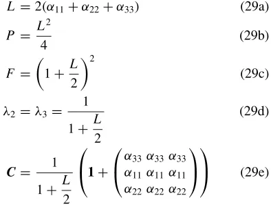
3.2.3 Numerical results Let us assume that the val-ues of the earthing and line resistances of a three-node network are S1 = 1.00 , S2 = 0.64 , S3 = 0.88 , R1 = 0.50 , R2 = 1.20 and R3 = 0.87 . These values are taken somewhat arbitrarily but they rep-resent typical values for a power network (Pirjola, 2009). Figure 1(a) presents the norm, given by Eq. (13), of the earthing currents obtained fromI =CJ, in which it is
as-sumed that thepecolumn matrixJ= ⎛ Fig. 1(a), altogether 32660 different column matricesJthat satisfy these conditions are used by changingJslightly and systematically between the runs of the calculation program. Figure 1(b) depicts the scalar product values betweenJand
a xed reference column matrixJref =
⎛ ⎝JJref 1ref 2
Jref 3
⎞
⎠also
nor-malised to unity and satisfying Eq. (6). The scalar product is de ned in the usual way as
In the present case N equals 3, but Eq. (32) is naturally applicable to other values ofN as well. Figure 1(b) shows that all possible column matricesJare really considered in the 32660 runs because the scalar product gets all values between −1 and +1. In other words, this means that J
(a)
(b)
Fig. 1. (a) Norm of the earthing GIC column matrix for a three-node network when thepecurrent column matrix is normalised to unity. The earthing resistances of the nodes areS1=1.00,S2=0.64andS3=0.88, and the line resistances areR1(line 1–2)=0.50,R2(line 2–3)=1.20
andR3(line 3–1)=0.87. Altogether 32660 runs of the calculation program are included by changing thepecurrent column matrix slightly and systematically between the runs and requiring that the sum of the elements of thepematrix is zero. The horizontal lines show two of the eigenvalues of the transfer matrix betweenpecurrents and earthing GIC (while the third eigenvalue equals one). (b) Scalar product between thepecurrent column matrices used in Fig. 1(a) for the 32660 runs and a fixed reference column matrix normalised to unity and having elements whose sum is zero.
should actually say thatJ and Jref are normalised to 1 A making [A2] be the unit of the scalar product.)
The eigenvalues of C are λ1 = 1, λ2 = 0.1869 and λ3 = 0.2978, the two latter of which are indicated by the horizontal lines in Fig. 1(a). We see that the norm of the earthing currents mostly lies between λ2 and λ3 but not always. In Fig. 1(a), the minimum and maximum of|I|
are 0.1867 and 0.2982, respectively. In practice, there is no difference betweenλ2and min(|I|)and betweenλ3and max(|I|). However, the positive differencesλ2−min(|I|) and max(|I|)−λ3are larger than the possible numerical in-accuracy in the computations. In the calculations presented in Fig. 1(a), altogether 0.79% and 6.66% of the|I|values are belowλ2 and aboveλ3, respectively. Thinking about practical GIC research,|I|gives a kind of an overall average
impact of GIC on transformers, and the present calculation indicates thatλ2andλ3determine the lower and upper limit of this impact. In this connection, it is necessary to empha-size that becauseJis normalised to unity the values of|I|
are quite small in Fig. 1(a). In a practical GIC case,|J|is much larger than 1 A, andλ2|J|andλ3|J|give the limits for
|I|. This comment also concerns the numerical calculations presented below in this paper.
Figures 2(a) and 2(b) show the same quantities as Figs. 1(a) and 1(b), respectively. Significant differences are, however, involved in the assumptions involved in Figs. 2(a) and 2(b) compared to Figs. 1(a) and 1(b). The resistances are now chosen by a randomisation procedure in reason-able ranges, which has resulted in the valuesS1 =0.96,
(a)
(b)
Fig. 2. (a) Norm of the earthing GIC column matrix for a three-node network when thepecurrent column matrix is normalised to unity. The earthing resistances of the nodes areS1=0.96,S2=1.10andS3=0.80, and the line resistances areR1(line 1–2)=1.62,R2(line 2–3)=0.97 andR3(line 3–1)=0.82. All these resistance values are chosen randomly in reasonable ranges. Thepecurrent column matrix is also determined randomly for every run of the calculation program requiring that the sum of the elements of thepematrix is zero. The total number of the runs is 100000. The horizontal lines show two of the eigenvalues of the transfer matrix betweenpecurrents and earthing GIC (while the third eigenvalue equals one). It is seen that the values of the norm of the earthing GIC cover the range between the two eigenvalues very accurately. (b) Scalar product between thepecurrent column matrices used in Fig. 2(a) for the 100000 runs and a fixed reference column matrix normalised to unity and having elements whose sum is zero. It is seen that the scalar product values cover the whole range from−1 to+1 very well.
R3=0.82to be used for Figs. 2(a) and 2(b). Thepe cur-rents J1,J2andJ3are also determined randomly for every run of the calculation program with the only constraints that they satisfy Eq. (6) andJis normalised to unity. The total number of the program runs is 100000. From Fig. 2(b) we notice that all scalar product values between−1 and+1 are encountered, which implies that all possible column matri-cesJare included in the computations. Looking at Fig. 2(b) carefully, it can be seen that values near±1 are a little bet-ter represented than values closer to zero. This is clearly a consequence of the fact that thecosine function, which is present in the scalar product, varies more slowly around±1 that at zero.
on the network.
Choosing the resistances to beS1 = 0.50,S2 =7.50 ,S3=0.75,R1=0.80,R2=1.20andR3=0.08 , we have the resonance case discussed in Section 3.2.2 since Eq. (28) are satis ed (with the products equalling 0.60 2). According to the theory, the eigenvaluesλ
2andλ3of
Care the same, and all column matrices J = ⎛ the values ofλ2andλ3in the cases investigated in Figs. 1(a) and 2(a) obviously results from the large resistanceS2. De-creasingS2by a factor of 4 and increasing R3by the same factor, i.e.S2 =1.875,R3=0.32, so that Eq. (28) still hold true, give a clearly larger valueλ2=λ3=0.18079.
3.3 Finnish 400 kV test model
Pirjola (2009) introduces an old version of the Finnish 400 kV power network valid in 1978 to 1979 as a test model for GIC calculation algorithms and programs. The geographical structure of today’s 400 kV grid in Finland is quite similar to the particular old version though not the same. Regarding GIC, an essential difference is produced by the installation of series capacitors in north-south lines (Elovaara, 2007). They block the ow of the dc-like GIC, which means that the Finnish 400 kV network consists of two separate parts as concerns GIC nowadays. (It should be noted that the reasons for the use of series capacitors are other than GIC mitigation.)
The Finnish 400 kV test model has 17 stations and 19 transmission lines, thus being complex enough to enable realistic GIC calculations but not too large to unnecessarily hamper the computations. The Cartesian at-Earth coordi-nates and (total) earthing resistances of the stations and the line resistances included in the test model are provided by Pirjola (2009). A special feature is that the earthing resis-tances of the two northwestern end stations are zero to ac-count for the galvanic connection of the grid to the Swedish 400 kV network. It is additionally assumed that the stations are distant enough, so the earthing impedance matrix is di-agonal. As Pirjola (2008) points out, it is not an essential limitation in practice. For reference information to the users of the test model, Pirjola (2009) also presents the values of GIC owing to (or from) the Earth at the stations and of GIC in the transmission lines when the test model is im-pacted by a northward or an eastward uniform geoelectric
eld of 1 V/km.
Figures 3(a) and 3(b) are similar to Figs. 2(a) and 2(b), except that the resistances are not chosen randomly but the correct test model values are used. A great difference is also, of course, thatC is a 17×17 matrix leading to 17 eigenvalues and implying that analytic solutions are impos-sible in practice. Figure 2(a) presents the norm ofI=CJ
(Eq. (13)) when the 17×1pecolumn matrix is determined in a random way, with the only constraints that |J| = 1 and Eq. (6) is satis ed, for each of the 100000 calcula-tion program runs. The horizontal lines in the gure in-dicate the eigenvalues. They are seen to satisfy the inequal-ities (12). The smallest and the largest (=1) eigenvalue
are plotted with thicker lines. We see that these extreme values clearly restrict the range of|I|. Actually|I| never reaches a value that is even very close to either of the ex-tremes in the 100000 runs performed. Looking at Fig. 3(b), we see that the random choices made in the runs do not cover all possibleJmatrices because the scalar product val-ues are concentrated in the range from about−0.6 to about +0.6 and never achieve values around±1. Mathematically, this may be understood by noting that we are operating in a 16-dimensional vector space. (One dimension of the 17-dimensional space is removed by the requirement that Eq. (6) is satis ed.) In Figs. 2(a) and 2(b), in which the vec-tor space is two-dimensional, 100000 runs of the program are suf cient, but we would need a much larger number of runs to be able to fully investigate|I|associated with the test model in question. Considering the Manitoba high-voltage network in Canada in a similar way (not shown here), we see that both the|I|values and the scalar products are con-centrated in even smaller ranges as the number of nodes is about ten times larger than in the test model.
An interesting detail concerning the test model is that the eigenvalueλ1 =1 is a double value, so it has two indepen-dent eigenvectors. Looking at the issue more carefully, we see that the eigenvectors correspond to situations where the
pecurrent has a non-zero value at one of the two northwest-ern zero-resistance stations and is zero elsewhere. Consid-ering such a case in terms of external injection of thepe cur-rents as mentioned in Section 2, the situation simply means that a current injected at a zero-resistance station directly ows into the Earth and nothing happens at other sites of the network. Thus, this is in accordance with what is men-tioned about thepecurrents associated with the eigenvalue equal to one in Section 3.1. It is easy to understand physi-cally but does not have any practical interest or importance. Besides Manitoba (Canada), similar calculations have also been performed for the high-voltage power networks in Brazil, China (ultra-high-voltage) and Southern Sweden. In every case, the inequalities (12) are valid as expected. Also otherwise, the results are comparable to those for the Finnish 400 kV test model. These additional results sup-port the above-mentioned conclusion valid for the Manitoba case that an increase of the number of nodes makes the plots corresponding to Figs. 3(a) and 3(b) concentrate in smaller ranges when the calculation program is run (only) 100000 times. A detail worth noting as well is that, similarly to the three-node network and the Finnish 400 kV test model, the valueλ = 1 (with a high accuracy) seems to be included in the set of eigenvalues in each calculation at least once. Finally, we emphasise that an earthing impedance matrix with non-zero off-diagonal elements (which is not the case for the three-node and test model cases) is included in the Manitoba and Southern Sweden computations. Because the conclusions are similar from all calculations, we thus ob-tain additional support to the fact that assuming the earthing impedance matrix to be diagonal is not a serious restriction in practice.
4.
Concluding Remarks
(a)
(b)
Fig. 3. (a) Norm of the earthing GIC column matrix for the Finnish 400 kV test model (see Pirjola, 2009) when thepecurrent column matrix is normalised to unity. Thepecurrent column matrix is determined randomly for every run of the calculation program requiring that the sum of the elements of thepematrix is zero. The total number of the runs is 100000. The horizontal lines show the eigenvalues of the transfer matrix betweenpe
currents and earthing GIC. It is seen that the values of the norm of the earthing GIC are clearly between the smallest eigenvalue and the largest (=1) eigenvalue, both of which are plotted with thicker lines. (b) Scalar product between thepecurrent column matrices used in Fig. 3(a) for the 100000 runs and a fixed reference column matrix normalised to unity and having elements whose sum is zero. It is seen that the scalar product values do not cover the range from−1 to+1, which means that the 100000 runs do not include all possiblepecurrent matrices.
using convenient matrix formulas whose input data con-sist of the horizontal geoelectric field at the Earth’s surface and of the network resistances and topology. This paper is focussed on the transfer matrix between the so-called “perfect-earthing” (pe) currents and GIC flowing between the Earth and the network. Thepecurrents depend on the geovoltages impacting the transmission lines and produced by the geoelectric field. The transfer matrix depends on the network resistances and topology in terms of an earthing impedance matrix and a network admittance matrix.
This paper provides a novel approach to the transfer ma-trix by considering its eigenvalues and eigenvectors. It is shown that either an eigenvalue equals one or the corre-sponding eigenvector satisfies the condition that the sum of
thepecurrents included in the particular eigenvector is zero, which implies that the amounts of pe currents flowing to and from the network are equal. The situation in which the eigenvalue equals one seems to be unimportant regarding practical GIC applications.
kV GIC test model also support that the eigenvalues lie be-tween zero and one. The same eigenvalue range is indicated by numerical calculations for other power grids as well.
Special attention is paid to the norm (=square root of the sum of the squares) of the earthing GIC owing between the Earth and the network. It is a quantity that gives an overall idea of the possibility of adverse impacts of GIC on a power grid since it is associated with GIC owing through transformers. If thepecurrent matrix is adjusted to have the norm equal to one, the norm of the earthing GIC seems to have the lower and upper limits equal to the smallest and largest (but=1) eigenvalue of the transfer matrix. This is an observation valid in practical GIC studies but not exactly. Without the normalisation of thepecurrent matrix to one, the lower and upper limits equal the smallest and largest eigenvalue multiplied by the norm of thepecurrents.
Acknowledgments. The author wishes to thank Dr. Ari Viljanen (Finnish Meteorological Institute) for many useful discussions on the topic of this paper. Thanks also go to all colleagues in the col-laboration concerning the Finnish, Swedish, Manitoba, Brazilian and Chinese power networks discussed in this paper.
References
Bolduc, L., GIC observations and studies in the Hydro-Qu´ebec power system,J. Atmos. Sol.-Terr. Phys.,64(16), 1793–1802, 2002.
Boteler, D. H. and R. J. Pirjola, Modelling geomagnetically induced cur-rents produced by realistic and uniform electric elds,IEEE Trans. Power Delivery,13(4), 1303–1308, 1998.
Boteler, D. H., R. J. Pirjola, and H. Nevanlinna, The effects of geomagnetic disturbances on electrical systems at the earth’s surface,Adv. Space Res.,
22(1), 17–27, 1998.
Elovaara, J., Finnish experiences with grid effects of GIC’s, inSpace Weather, Research towards Applications in Europe, edited by J. Lilen-sten, Chapter 5.4, 311–326, Astrophysics and Space Science Library, 344, ESA, COST 724, Springer, 2007.
Kappenman, J. G., Geomagnetic disturbances and impacts upon power system operation, inThe Electric Power Engineering Handbook, 2nd edition, edited by L. L. Grigsby, Chapter 16, 16-1–16-22, CRC Press/IEEE Press, 2007.
Lanzerotti, L. J., D. J. Thomson, and C. G. Maclennan, Engineering issues in space weather, in Modern Radio Science 1999, edited by M. A. Stuchly, 25–50, International Union of Radio Science (URSI), Oxford University Press, 1999.
Lehtinen, M. and R. Pirjola, Currents produced in earthed conductor net-works by geomagnetically-induced electric elds,Ann. Geophys.,3(4), 479–484, 1985.
Molinski, T. S., Why utilities respect geomagnetically induced currents,J. Atmos. Sol.-Terr. Phys.,64(16), 1765–1778, 2002.
Pirjola, R., Review on the calculation of surface electric and magnetic elds and of geomagnetically induced currents in ground-based tech-nological systems,Surv. Geophys.,23(1), 71–90, 2002.
Pirjola, R., Effects of interactions between stations on the calculation of geomagnetically induced currents in an electric power transmission sys-tem,Earth Planets Space,60(7), 743–751, 2008.
Pirjola, R., Properties of matrices included in the calculation of geomag-netically induced currents (GICs) in power systems and introduction of a test model for GIC computation algorithms,Earth Planets Space, 61(2), 263–272, 2009.
Viljanen, A., A. Pulkkinen, O. Amm, R. Pirjola, T. Korja, and BEAR Working Group, Fast computation of the geoelectric eld using the method of elementary current systems and planar Earth models,Ann. Geophys.,22(1), 101–113, 2004.