Numerical algorithms for multidimensional time fractional wave equation of distributed order with a nonlinear source term

R E S E A R C H

Open Access

Numerical algorithms for

multidimensional time-fractional wave

equation of distributed-order with a

nonlinear source term

Jiahui Hu

_{, Jungang Wang}

_{and Yufeng Nie}

*_{Correspondence:}

[email protected]

1_{Research Center for Computational} Science, Northwestern

Polytechnical University, Xi’an, China Full list of author information is available at the end of the article

Abstract

Fractional differential equations (FDEs) of distributed-order are important in depicting the models where the order of differentiation distributes over a certain range. Numerically solving this kind of FDEs requires not only discretizations of the temporal and spatial derivatives, but also approximation of the distributed-order integral, which brings much more difficulty. In this paper, based on the mid-point quadrature rule and composite two-point Gauss–Legendre quadrature rule, two finite difference schemes are established. Different from the previous works, which concerned only one- or two-dimensional problems with linear source terms, time-fractional wave equations of distributed-order whose source term is nonlinear in two and even three dimensions are considered. In addition, to improve the computational efficiency, the technique of alternating direction implicit (ADI) decomposition is also adopted. The unique solvability of the difference scheme is discussed, and the unconditional stability and convergence are analyzed. Finally, numerical experiments are carried out to verify the effectiveness and accuracy of the algorithms for both the two- and three-dimensional cases.

MSC: 35R11; 65M06; 65M12

Keywords: Time-fractional wave equation of distributed-order; ADI finite difference scheme; Nonlinear source term; Stability; Convergence

1 Introduction

The idea of distributed-order differential equation was first presented by Caputo for mod-eling the stress–strain behavior of an anelastic medium in [5] in the 1960s. Unlike the differential equations with the single-order fractional derivative and those with sums of fractional derivatives, i.e., multi-term FDEs, the distributed-order differential equations are derived by integrating the order of differentiation over a given range [1]. This can be regarded as a generalization of the aforementioned two classes of FDEs. Such FDEs are typically applied in a retarding sub-diffusion process, during which a plume of particles spreads at a logarithmic rate, and eventually the ultraslow diffusion is generated (see [8, 22,29]). For example, the fractional Langevin equation of distributed-order was originally proposed for modeling the kinetics of retarding sub-diffusion, and then was found

cient in simulating the strongly anomalous ultraslow diffusion, where the mean square displacement grew as a power of logarithm of time [11]. Also, for optimal control prob-lems, the integer order derivative is replaced by that of a distributed-order so as to capture delays of distinct sources. In [35], considering the optimal control problems with dynam-ics described by ordinary distributed-order fractional differential equations, the general-ized necessary conditions were derived. Then an efficient numerical scheme was proposed and applied to solve an unconstrained convex distributed optimal control problem which is governed by the distributed-order fractional differential equations. In [34], a general formulation for the fractional optimal control problems with distributed-order fractional derivatives was presented, and a Legendre spectral collocation scheme for solving the de-rived boundary value problem was presented along with error analysis. Besides, there are also other various research fields involving the distributed-order FDEs, such as control and signal processing [20], modeling dielectric induction and diffusion [6], identification of systems [19], and so forth.

Recently, there have been many important progresses in the research of analytical solu-tions of distributed-order FDEs. For researching the kinetic description of anomalous dif-fusion and relaxation phenomena, Chechkin et al. [7] presented a diffusion-like equation with time fractional derivative of distributed-order, the authors also proved the positivity of the solutions and established the relation to the continuous-time random walk theory. Atanackovic et al. analyzed a Cauchy problem for a time distributed-order diffusion-wave equation by means of the theory of an abstract Volterra equation in [2]. In view of the fundamental solution of the Cauchy problem of the one-dimensional distributed-order diffusion-wave equation, Gorenflo et al. gave the interpretation that it is a probability density function of the space variable xevolving in timetin the transform domain by employing the technique of the Fourier and Laplace transforms [18]. Using the Laplace transform method, Li et al. [23] investigated the asymptotic behavior of solutions to the initial-boundary-value problem for the distributed-order time-fractional diffusion equa-tions.

was applied to improve the approximate accuracy [17]. In [13], the authors handled the one- and two-dimensional distributed-order diffusion equations by employing a weighted and shifted Grünwald–Letnikov formula to derive several high-order difference schemes. A distributed-order time and Riesz space-fractional Schrödinger equation was simulated by developing a new numerical approach in [4]. The considered problem was first trans-formed into a system of distributed-order fractional differential equations by employing the Jacobi–Gauss–Lobatto collocation method, and then the derived system was solved by a spectral method based on Jacobi–Gauss–Radau collocation method. In terms of the time distributed-order diffusion-wave equations, most of the work considers the one-dimensional case, and the integrating range of the order of time derivative is the interval [0, 1], which is named the time distributed-order diffusion equation. When the order of the time derivative is distributed over the interval [1, 2], it is called the time distributed-order wave equation. Ye et al. derived and analyzed a compact difference scheme for a distributed-order time-fractional wave equation in [32].

In this work, we propose efficient finite difference schemes for solving the two-and three-dimensional time-fractional wave equations of distributed-order, respectively, where a nonlinear source term is considered. As far as we know, the relevant literature is rather limited. Gao et al. investigated ADI difference schemes for two-dimensional time distributed-order diffusion equations [14,16]. In [14], Grünwald formula was employed and ADI difference scheme as well as compact ADI difference scheme were derived. The extrapolation method was also applied to obtain the improved approximate accuracy. In [16], the authors proposed two ADI difference schemes and proved that they were uncon-ditionally stable and convergent in a discreteL1(L∞) norm. Based on the weighted and shifted Grünwald–Letnikov formula, they also developed two ADI difference schemes for solving the two-dimensional time distributed-order wave equations [15]. Abbaszadeh et al. solved the two-dimensional distributed order time-fractional diffusion-wave equation by combining the ADI approach with the interpolating element-free Galerkin method, where the time derivatives was discretized by a finite difference scheme [1]. Using the same time approximation method, and based on the shape functions of reproducing ker-nel particle method, a novel element-free Galerkin approach was proposed for solving 2D fractional Tricomi-type equation with Robin boundary condition [9]. Additionally, real-izing the widespread use of the differential equations with nonlinear source terms [27, 31], Morgado et al. presented an implicit difference scheme for time distributed-order diffusion equation with a nonlinear source term in one dimension [24].

The structure of the rest of this work is as follows. In Sect.2, based on the mid-point quadrature rule and composite two-point Gauss–Legendre quadrature rule, two differ-ence schemes for the two-dimensional problem are constructed and described in details. In Sect.3, the solvability, stability and convergence of the derived difference schemes are discussed. Section4gives the description of ADI forms of the proposed schemes. We es-tablish the ADI finite difference schemes for the three-dimensional problem in Sect.5. Numerical results are illustrated in Sect.6to confirm the effectiveness and accuracy of our methods for both the two- and three-dimensional cases, and some conclusions are drawn in the last section.

2 The derivation of the schemes for the two-dimensional problem

We consider the two-dimensional problem first. The two-dimensional time-fractional wave equation of distributed-order with a nonlinear source term along with its initial and boundary conditions can be written as

2 1

p(β)C₀Dβtu(x,y,t)dβ=

∂2u(x,y,t) ∂x2 +

∂2u(x,y,t) ∂y2 +f

x,y,t,u(x,y,t),

(x,y)∈Ω,t∈(0,T], (1)

u(x,y,t) =φ(x,y,t), (x,y)∈∂Ω,t∈[0,T], (2)

u(x,y, 0) =ψ1(x,y), ut(x,y, 0) =ψ2(x,y), (x,y)∈Ω, (3)

whereΩ= (0,L1)×(0,L2), and∂Ωis the boundary ofΩ. The fractional derivativeC0D

β

tv(t)

in (1) is given in the Caputo sense

C

0D

β

tv(t) = ⎧ ⎪ ⎪ ⎨ ⎪ ⎪ ⎩

∂v(t)

∂t –

∂v(0)

∂t , β= 1,

1

Γ(2–β)

t

0(t–ξ) 1–β ∂2v(ξ)

∂ξ2 dξ, 1 <β< 2, ∂2v(t)

∂t2 , β= 2,

the functionp(β) serves as a weight for the order of differentiation and is such thatp(β) > 0 and ₁2p(β)dβ=c0> 0. We assume thatp(β),φ(x,y,t),ψ1(x,y),ψ2(x,y) andf(x,y,t,u) are

continuous, and the nonlinear source termfsatisfies the Lipschitz condition with respect tou:

f(x,y,t,u1) –f(x,y,t,u2)≤Lf|u1–u2|, (4)

whereLf is a positive constant.

using the discrete energy method, we prove that the derived numerical schemes are un-conditionally stable and convergent in the discreteL2 _{norm, and then the ADI forms of}

the proposed schemes are given for computing.

The rest of this section focuses on deriving the finite difference scheme for the problem (1)–(3).

LetM1,M2andNbe positive integers, andh1=L1/M1,h2=L2/M2andτ=T/Ndenote

the uniform sizes of spatial grid and time step, respectively. Then a spatial and temporal partition can be defined asxi=ih1fori= 0, 1, . . . ,M1,yj=jh2forj= 0, 1, . . . ,M2andtn=nτ

forn= 0, 1, . . . ,N. Denote

Ωh=

(xi,yj)|1≤i≤M1– 1, 1≤j≤M2– 1

,

∂Ωh=

(xi,yj)|i= 0 ori=M1orj= 0 orj=M2

, Ω¯h=Ωh∪∂Ωh,

Ωτ ={tn|tn=nτ, 0≤n≤N}.

Then the domainΩ¯ ×[0,T] is covered byΩ¯h×Ωτ. Letu={un_ij|0≤i≤M1, 0≤j≤

M2, 0≤n≤N}represent a grid function onΩ¯h×Ωτ. We introduce the following nota-tions:

un– 1 2 ij =

1 2

un_ij+un_ij–1, δtu n–1₂

ij =

1 τ

un_ij–un_ij–1, δxun_i–1

2,j= 1

h1

un_ij–un_i–1,j, δ2_xun_ij= 1

h1

δxun_i+1 2,j–

δxun_i–1 2,j

,

δyun_i,j–1 2

= 1

h2

un_ij–un_i,j–1, δ_y2un_ij= 1

h2

δxun_i,j+1 2

–δxun_i,j–1 2

,

and

Δhuij=δ2xuij+δy2uij.

Consider Eq. (1) at the point (xi,yj,tn), which can be written as

2 1

p(β)C₀Dβtu(xi,yj,tn)dβ

=∂

2_u(xi,yj,tn)

∂x2 +

∂2_u(xi,yj,tn)

∂y2 +f

xi,yj,tn,u(xi,yj,tn). (5)

Taking an average of Eq. (5) at time instantst=tnandt=tn–1, we obtain the following

equations:

1 2

2

1

p(β)C₀Dβ_tu(xi,yj,tn)dβ+ 2

1

p(β)C₀Dβ_tu(xi,yj,tn–1)dβ

=1 2

∂2u(xi,yj,tn) ∂x2 +

∂2u(xi,yj,tn–1)

∂x2

+1 2

∂2u(xi,yj,tn) ∂y2 +

∂2u(xi,yj,tn–1)

∂y2

+1 2

fxi,yj,tn,u(xi,yj,tn)

+fxi,yj,tn–1,u(xi,yj,tn–1)

Denote byU_ijn=u(xi,yj,tn) the grid functions onΩ¯h×Ωτ with 0≤i≤M1, 0≤j≤M2,

Firstly, we discretize the integral term in (7). Here the mid-point quadrature rule and the composite two-point Gauss–Legendre quadrature rule are employed, respectively. Suppose p(β)∈C4_{[1, 2],} C

approximating the integral in (7), we are left with the following multi-term time-fractional wave equation:

whereR1=O(Δβ2). While using the composite two-point Gauss–Legendre quadrature

rule, we arrive at an analogous equation as follows:

Δβ Here, we present the procedure for (8), and the technique used for (9) is similar.

Supposeu(x,y,t)∈Cx4,4,3,y,t(Ω¯ ×[0,T]). According to Theorem 8.2.5 in [30], the Caputo

ij , 1 <βl< 2 has the fully discrete difference scheme

and

In the meantime, the central difference quotient is used to approximate the second order derivatives in (8). Then we obtain

Δβ

lowing manner to avoid a system of nonlinear equations when computing:

In the following, we discuss the necessary estimate ofRn– 1 2

ij . From (11), we can deduce that

there exists a positive constantC1such that

–

K

l=1

Δβp(βl)Rl2

≤C1τ1+

1 2Δβ

K

l=1

Δβp(βl).

Since

K

l=1

Δβp(βl)∼ 2

1

p(β)dβ=c0,

we get

K

l=1

Δβp(βl)≤C2,

whereC2is a positive constant. Thus there is a positive constantC3such that

Rn– 1 2 ij ≤C3

τ1+12Δβ_+h2

1+h22+Δβ2

.

Besides, Eq. (15) implies that

Rn– 1 2

ij ≤C4τ,

whereC4is a positive constant.

To establish an efficient numerical scheme, the procedure below is needed. Denote

μ=Δβ

K

l=1

p(βl)

1 τβl_{Γ(3 –βl)}.

Since

Δβ

K

l=1

p(βl)

1 τβ_{lΓ(3 –β}

l)

∼

2 1

p(β) 1 τβ_{Γ(3 –β)}dβ

= p(β ∗₎

Γ(3 –β∗)

2 1

1 τβdβ

= p(β ∗₎

Γ(3 –β∗) 1 –τ τ2_|lnτ|,

it can be concluded that

μ= 1

Whenτ is sufficiently small,|lnτ| ≤Cτ–ε_{holds for any positive and smallε. Therefore,} the termO(τ2|lnτ|) is almost the same asO(τ2) whenτ is sufficiently small. Adding the high order term

Rn–

whereC5is a positive constant. Also, for the initial and boundary conditions, we have

and

φn_ij=φ(xi,yj,tn), (i,j)∈γ, 0≤n≤N.

Starting the procedure by Eq. (9), we have the scheme for solving (1)–(3) as

Δβ 2

K

l=1

pβ_l(1) τ

1–β_l(1) Γ(3 –β_l(1))

a(β

(1)

l )

0 δtu n–1₂

ij – n–1

k=1

a(β

(1)

l )

n–k–1–a (β_l(1))

n–k

δtuk– 1 2 ij

–a(β (1)

l )

n–1 (ψ2)ij

+Δβ 2

K

l=1

pβ_l(2) τ

1–β_l(2) Γ(3 –β_l(2))

a(β

(2)

l )

0 δtu n–1₂

ij

–

n–1

k=1

a(β

(2)

l )

n–k–1–a (β_l(2))

n–k

δtuk– 1 2 ij –a

(β_l(2))

n–1 (ψ2)ij

+ τ 4μδ

2

xδ2y un

ij–unij–1

τ

=δ_x2un– 1 2 ij +δ2yu

n–12 ij +f

xi,yj,tn–1,unij–1

,

1≤i≤M1– 1, 1≤j≤M2– 1, 1≤n≤N, (22)

u0_ij= (ψ1)ij, 1≤i≤M1– 1, 1≤j≤M2– 1, (23)

un_ij=φ_ijn, (i,j)∈γ, 0≤n≤N, (24)

where the omitted remainder isO(τ+h2

1+h22+Δβ4), and

μ=Δβ 2

K

l=1

pβ_l(1) 1 τβ(1)l _Γ(3 –_β(1)

l )

+Δβ 2

K

l=1

pβ_l(2) 1 τβl(2)_Γ(3 –_β(2)

l )

.

3 Analysis of the difference scheme

In this section, the analysis of scheme (19)–(21) is carried out, and that for scheme (22)– (24) is similar.

3.1 Unique solvability

In this subsection, the unique solvability of scheme (19)–(21) is proved.

Theorem 1 The finite difference scheme(19)–(21)is uniquely solvable.

Proof Letun_={un

ij|0≤i≤M1, 0≤j≤M2}. It can be seen that the value ofu0is uniquely

determined by (20) and (21). Suppose the values ofu0,u1, . . . ,un–1have been uniquely de-termined. To show that the linear system of equations (19) and (21) has a unique solution, it is sufficient to prove that the corresponding homogeneous one, namely

μun_ij–1 2Δhu

n ij+

1 4μδ

2

xδy2unij= 0, 1≤i≤M1– 1, 1≤j≤M2– 1, (25)

un_ij= 0, i= 0 ori=M1orj= 0 orj=M2, (26)

Multiplying (25) byh1h2unij, summing overifrom 1 toM1– 1 and overjfrom 1 toM2– 1,

we have

μun2+1 2u

n2₊ 1

4μδxδyu

n2_{= 0. (27)}

Equation (27) implies un _{= 0. Combining with (26) this yieldsu}n_{= 0.}

According to the principle of mathematical induction, the proof is completed.

3.2 Stability

In this subsection we focus on showing the unconditional stability of the difference scheme (19)–(21). We introduce some auxiliary definitions and useful results which will also be used when the convergence is considered.

Denote the space of grid functions onΩ¯hby

Vh=v|v=vij|(xi,yj)∈ ¯Ωh

andvij= 0 if (xi,yj)∈∂Ωh

.

For any grid function v∈Vh, the following discrete norms and Sobolev seminorm are introduced:

v =

_h1h2M1–1 i=1

M2–1 j=1

|vij|2_{, δ}

xδyv = _h1h2M1

i=1

M2

j=1

|δxδyvi–₂1,j–1₂|2,

δxv = _h1h2M1

i=1

M2–1

j=1

|δxvi–1₂,j|2, δyv =

_h1h2M1–1 i=1

M2

j=1

|δyvi,j–1₂|2,

Δhv =

_h1h2M1–1 i=1

M2–1 j=1

|Δhvij|2_, |_v| 1=

δxv 2_{+ δyv} 2_.

Lemma 1([28]) For any grid function v∈Vh, v ≤ √L1L2

6(L2₁+L2₂)|v|1.

Lemma 2([30]) For any grid function v∈Vh,|v|1≤√L1L2 6(L21+L22)

Δhv .

Lemma 3([30]) For any G={G1,G2,G3, . . .}and q,we have

s

n=1

b0Gn–

n–1

k=1

(bn–k–1–bn–k)Gk–bn–1q

Gn

≥t1–s α

2 τ

s

n=1

G2_n– t

2–α

s

2(2 –α)q

2_{, s= 1, 2, 3, . . . ,}

where

bl= τ

2–α 2 –α

(l+ 1)2–α–l2–α, l= 0, 1, 2, . . . .

Lemma 4([26]) Assume that knand pnare nonnegative sequences,and the sequenceΦn

ijis an approximation solution ofunij, which is the exact solution of the

scheme (19)–(21). Also, suppose that (ψ1)ij and (ψ2)ij are approximations to (ψ1)ijand

(ψ2)ij, respectively. Denoteεijn=unij–unij, 0≤i≤M1, 0≤j≤M2, 0≤n≤N. Then we have

the perturbation error equations

Δβ unconditionally stable.

Multiplying (29) byh1h2τ δtε n–1₂

ij , summing over ifrom 1 toM1– 1, overjfrom 1 to

M2– 1, and overnfrom 1 tos, we analyze each term in the resulted equation. Firstly, by

Lemma3, we have

Subsequently, using the discrete Green formula, we get the following two equations:

Analogous to (32), we also obtain

From Eqs. (30)–(34), the following inequality holds:

δxεs

Finally, applying Lemma4, we derive

εn2≤

3.3 Convergence

In this part, the convergence of the difference approximation is discussed. Notice that ifU_ijn

is the exact solution of the system (1)–(3) andun

ijis the numerical solution of the difference

scheme (19)–(21), then the error is denoted as

τ

Then for the term containing the remainders, it can be deduced that

i.e.,

From Lemma1, we obtain

en2≤ L

Therefore, by using Lemma4, we have

_en2_≤ L31L32

This completes the proof.

4 Description of the ADI scheme

For ease of computation, the ADI scheme is developed in this section. Considering Eqs. (19)–(21), and noticinga(βl)

Let

Then we have the ADI form of difference scheme (19)–(21), and the procedure can be executed as follows:

At each time instance t=tn(1≤n≤N), firstly, for all fixedy=yj(1≤j≤M2– 1),

by solving a set ofM1– 1 equations at the mesh pointsxi (1≤i≤M1– 1), we get the

intermediate solutionu∗_ij:

⎧

solutionu∗_ijis derived:

5 Three-dimensional problem

In what follows, we present numerical schemes for the three-dimensional problem. Consider the three-dimensional time-fractional wave equation of distributed-order with a nonlinear source term along with its initial and boundary conditions:

2 1

p(β)C₀Dβtu(x,y,z,t)dβ

=∂

2_u(x,y,z,t)

∂x2 +

∂2u(x,y,z,t) ∂y2 +

∂2u(x,y,z,t) ∂z2

+fx,y,z,t,u(x,y,z,t), (x,y,z)∈Ω,t∈(0,T], (47)

u(x,y,z,t) =φ(x,y,z,t), (x,y,z)∈∂Ω,t∈[0,T], (48)

u(x,y,z, 0) =ψ1(x,y,z), ut(x,y,z, 0) =ψ2(x,y,z), (x,y,z)∈Ω, (49)

whereΩ= (0,L1)×(0,L2)×(0,L3), and∂Ω is the boundary ofΩ. We still assume that

p(β),φ(x,y,z,t),ψ1(x,y,z),ψ2(x,y,z) andf(x,y,z,t,u) are continuous, and the nonlinear

source termf satisfies a Lipschitz condition of the form

f(x,y,z,t,u1) –f(x,y,z,t,u2)≤Lf|u1–u2|, (50)

whereLf is a positive constant.

LetM1, M2, M3 andN be positive integers, andhi=Li/Mi (i= 1, 2, 3) and τ =T/N

represent the uniform step sizes in spatial and temporal directions, respectively. Denote

Ωh=

(xi,yj,zm)|1≤i≤M1– 1, 1≤j≤M2– 1, 1≤m≤M3– 1

,

∂Ωh=

(xi,yj,zm)|i= 0 ori=M1orj= 0 orj=M2orm= 0 orm=M3

,

¯

Ωh=Ωh∪∂Ωh,

Ωτ ={tn|tn=nτ, 0≤n≤N}.

Then the partition ofΩ¯×[0,T] isΩ¯h×Ωτ. TakeUn

ijm=u(xi,yj,zm,tn), the grid functions onΩ¯h×Ωτ, with 0≤i≤M1, 0≤j≤M2,

0≤m≤M3, 0≤n≤N. Similar to the derivation of Eq. (14), we get the equation

Δβ

K

l=1

p(βl)

τ1–βl Γ(3 –βl)

a(βl)

0 δtU

n–12 ijm –

n–1

k=1

a(βl)

n–k–1–a (βl)

n–k

δtUk– 1 2 ijm

–a(βl)

n–1ψ2(xi,yj,zm)

=δ_x2Un– 1 2 ijm +δ2yU

n–1₂

ijm +δz2U n–1₂

ijm +f

xi,yj,zm,tn–1,Uijmn–1

+Rn– 1 2 ijm +R

n–1₂

ijm , (51)

where there exist positive constantsC6andC7such that

Rn– 1 2 ijm ≤C6

τ1+12Δβ_+h2

1+h22+h23+Δβ2

and

Rn– 1 2

ijm ≤C7τ.

Adding the high order term

Rn–

whereC8is a positive constant. For the initial and boundary conditions, we have

U_ijm0 =ψ1(xi,yj,zm), (xi,yj,zm)∈Ωh, (54) U_ijmn =φ(xi,yj,zm,tn), (xi,yj,zm)∈∂Ωh, 0≤n≤N. (55)

Letun

ijmbe a numerical approximation tou(xi,yj,zm,tn). Neglecting the small termsR n–1₂

difference scheme for (47)–(49) as follows:

1≤i≤M1– 1, 1≤j≤M2– 1, 1≤m≤M3– 1, 1≤n≤N, (56)

u0_ijm= (ψ1)ijm, 1≤i≤M1– 1, 1≤j≤M2– 1, 1≤m≤M3– 1, (57)

un_ijm=φ_ijmn , (i,j,m)∈γ =(i,j,m)|(xi,yj,zm)∈∂Ωh

, 0≤n≤N, (58)

where

(ψ1)ijm=ψ1(xi,yj,zm), (ψ2)ijm=ψ2(xi,yj,zm),

1≤i≤M1– 1, 1≤j≤M2– 1, 1≤m≤M3– 1

and

φn_ijm=φ(xi,yj,zm,tn), (i,j,m)∈γ, 0≤n≤N.

By defining the discrete norms and Sobolev seminorm corresponding to the three-dimensional problems, we can prove that Lemmas1and2are available for the cuboidal domain. The theoretical analysis for the three-dimensional problem can be performed in a similar manner as of the two-dimensional case in Sect.3, though it is much more compli-cated. For the sake of briefness, we won’t repeat it and list the theoretical results directly. Hence, as generalizations of Theorems1,2and3, we have the following conclusions.

Theorem 4 The finite difference scheme(56)–(58)is uniquely solvable.

Theorem 5 If condition(50)is satisfied,then the difference scheme(56)–(58)is uncondi-tionally stable.

Theorem 6 Suppose that the continuous problem(47)–(49)has a solution u(x,y,z,t)∈

C4,4,4,3

x,y,z,t(Ω¯×[0,T])and condition(50)is satisfied.Then there is a positive constant C such that

en≤Cτ+h2₁+h2₂+h2₃+Δβ2.

For ease of implementation, we adopt the following ADI scheme when computing. At each time instancet=tn (1≤n≤N), firstly, for all fixedy=yj (1≤j≤M2– 1)

andz=zm (1≤m≤M3– 1), solving a set of M1– 1 equations at the mesh points xi

(1≤i≤M1– 1), the first intermediate solutionu∗∗ijmis given as: ⎧

⎪ ⎪ ⎪ ⎪ ⎪ ⎪ ⎪ ⎪ ⎪ ⎪ ⎪ ⎪ ⎪ ⎨ ⎪ ⎪ ⎪ ⎪ ⎪ ⎪ ⎪ ⎪ ⎪ ⎪ ⎪ ⎪ ⎪ ⎩

(√3_μI– 1

2μ23 δ2_x)u∗∗_ijm

= (√3_μI+ 1

2μ 2 3

δ2_x)(√3_μI+ 1

2μ 2 3

δ_y2)(√3_μI+ 1

2μ 2 3

δ_z2)un–1

ijm

+Δβ!K_l=1p(βl)_τβ_lΓ1_(3–β

l)[

!n–1

k=1(a (β_l)

n–k–1–a (β_l)

n–k)(ukijm–ukijm–1)

+τa(βl)

n–1(ψ2)ijm]

+f(xi,yj,zm,tn–1,unijm–1), 1≤i≤M1– 1,

u∗∗_0jm= (√3_μI– 1

2μ23

δ_y2)u∗_0jm, u∗∗_M 1jm= (

3 √_μI– 1

2μ23 δ2_y)u∗_M

1jm;

afterwards, for all fixedz=zm (1≤m≤M3– 1) andx=xi(1≤i≤M1– 1), by solving a

set ofM2– 1 equations at the mesh pointsyj(1≤j≤M2– 1), the second intermediate

solutionu∗_ijmcan be obtained:

⎧

Also, by employing the composite two-point Gauss–Legendre quadrature rule, the ADI scheme for the three-dimensional problem is obtained, and it is described as following:

At each time instancet=tn (1≤n≤N), firstly, for all fixedy=yj (1≤j≤M2– 1)

solutionu∗_ijmcan be obtained:

6 Numerical results

In this section, numerical examples are given to demonstrate the availability of the pro-posed schemes and verify the theoretical results, including convergence orders and nu-merical stability. Both the discreteL2andL∞norms are taken to measure the numerical errors. Denote

eN_L2:=

_M3–1

m=1

M2–1 j=1

M1–1 i=1

U_ijmN –uN_ijm2h1h2h3

1 2 ,

and

eN_L∞:= max

1≤m≤M3–1,1≤j≤M2–1,1≤i≤M1–1

U_ijmN –uN_ijm.

Example1 We consider

2 1

Γ(4 –β)C₀Dβ_tu(x,y,t)dβ

=∂

2_u(x,y,t)

∂x2 +

∂2_u(x,y,t)

∂y2 +sinxsiny

2t3+ 2t+ 4+6t

2_{– 6t}

lnt

–t3+ 2t+ 42sin2xsin2y+u2(x,y,t), 0 <t≤1/2, (x,y)∈Ω= (0,π)×(0,π),

u(x,y,t) = 0, (x,y)∈∂Ω, 0≤t≤1/2,

u(x,y, 0) = 4sinxsiny, ut(x,y, 0) = 2sinxsiny, (x,y)∈Ω,

whose analytical solution is known and is given by

u(x,y,t) =t3+ 2t+ 4sinxsiny.

A comparison of the numerical and exact solutions for Example1is presented in Fig.1. It can be seen that they agree well with each other.

Table1records the numerical accuracy of scheme (43)–(44) and scheme (45)–(46) in time for Example1. Let the step sizesh1,h2, andΔβbe fixed and small enough such that

the dominating error arises from the approximation of the time derivatives. In the current test, the fixed step sizes are set ash1=h2=π/500,Δβ= 1/160 for scheme (43)–(44), and

h1=h2=π/100,Δβ= 1/10 for scheme (45)–(46), respectively. Varying the step size in

time, the numerical errors in the discreteL2_{norm and the associated convergence orders}

are shown in this table, which can be found in agreement with the theoretical analysis. In Table2, the fixed and small enough step sizes in space are taken, and an optimal step size ratio in time and distributed order is adopted for difference scheme (43)–(44). As Δβ andτ vary, we compute the errors and convergence orders listed in the table, which indicate that the convergence orders in time and distributed order are about one and two, respectively. It is in accord with the theoretical analysis.

Figure 1Exact solution (a) and numerical solution (b) atT= 0.5 with meshh1=h2=₆₄π,Δβ=₆₄1 and τ=₄₀₉₆1 by scheme (43)–(44) (Example1)

Table 1 Errors and convergence orders of scheme (43)–(44) and scheme (45)–(46) in temporal direction (Example1)

τ Scheme (43)–(44) Scheme (45)–(46)

eN _L2 Order CPU time eN _L2 Order CPU time

1/10 0.1225 – 0.1882 s 0.1222 – 0.0129 s

1/20 0.0634 0.9502 0.4328 s 0.0632 0.9512 0.0411 s

1/40 0.0326 0.9596 1.0168 s 0.0324 0.9639 0.0580 s

1/80 0.0167 0.9650 2.6598 s 0.0164 0.9823 0.1016 s

1/160 0.0085 0.9743 8.4336 s 0.0082 1.0000 0.2387 s

Table 2 Errors and convergence orders of scheme (43)–(44) withh1=h2=₅₀₀π , and an optimal step

size ratio forτandΔβ(Example1)

τ Δβ eN

L2 Order e

N

L∞ Order CPU time

1/100 1/10 0.0133 – 0.0093 – 3.7889 s

1/400 1/20 0.0034 1.9678 0.0024 1.9542 44.8796 s

1/1600 1/40 8.6411e–04 1.9762 6.0481e–04 1.9885 654.4187 s

1/6400 1/80 2.1076e–04 2.0365 1.4751e–04 2.0357 2 h 48 m 8 s

Table 3 Errors and convergence orders of scheme (43)–(44) with an optimal step size ratio forτ,h1, h₂andΔβ(Example1)

τ h1=h2 Δβ eN L2 Order e

N

L∞ Order CPU time

1/64 π/2 1/8 0.7230 – 0.4602 – 0.0816 s

1/256 π/4 1/16 0.1689 2.0978 0.1195 1.9453 0.0483 s

1/1024 π/8 1/32 0.0426 1.9872 0.0301 1.9892 0.2603 s

1/4096 π/16 1/64 0.0107 1.9932 0.0075 2.0048 5.4613 s

1/16,384 π/32 1/128 0.0027 1.9866 0.0019 1.9809 166.2940 s

1/65,536 π/64 1/256 6.6801e–04 2.0150 4.7098e–04 2.0123 1 h 46 m 27 s

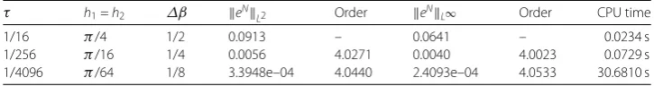
Table 4 Errors and convergence orders of scheme (45)–(46) with an optimal step size ratio forτ,h1, h2andΔβ(Example1)

τ h1=h2 Δβ eN L2 Order eN L∞ Order CPU time

1/16 π/4 1/2 0.0913 – 0.0641 – 0.0234 s

1/256 π/16 1/4 0.0056 4.0271 0.0040 4.0023 0.0729 s

order, respectively. One can conclude from Table3that the convergence orders of scheme (43)–(44) with respect to time, space and distributed order are about one, two and two. While in Table4, it can be found that the convergence orders of scheme (45)–(46) in time, space and distributed order are approximately one, two and four. These results agree well with the theoretical convergence orders.

Example2 We now consider

2 1

Γ(4 –β)C₀Dβtu(x,y,z,t)dβ

=∂

2_u(x,y,z,t)

∂x2 +

∂2u(x,y,z,t) ∂y2 +

∂2u(x,y,z,t) ∂z2

+sinxsinysinz

3t3+ 2t+ 4+6t

2_{– 6t}

lnt

–t3+ 2t+ 42sin2xsin2ysin2z+u2(x,y,z,t), 0 <t≤1/2, (x,y,z)∈Ω= (0,π)×(0,π)×(0,π),

u(x,y,z,t) = 0, (x,y,z)∈∂Ω, 0≤t≤1/2,

u(x,y,z, 0) = 4sinxsinysinz, ut(x,y,z, 0) = 2sinxsinysinz, (x,y,z)∈Ω,

whose analytical solution is known and is given by

u(x,y,z,t) =t3+ 2t+ 4sinxsinysinz.

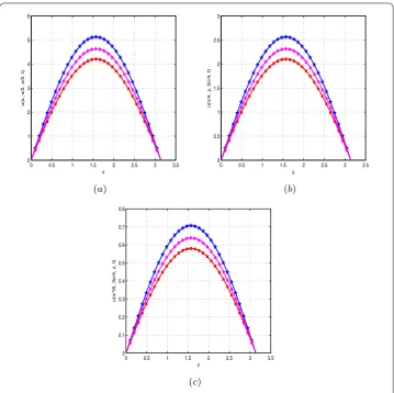
Comparisons of numerical solutions with the exact solutions for Example2are shown in Figs.2and3. In Fig.2(a), lety=z=π

2. Then the numerical and exact solutions along

thex-axis for different time instances are plotted with meshh1=h2=h3=₃₂π,Δβ=₃₂1,

andτ =₁₀₂₄1 . Based on the same partition, fixingx=π₄,z=3₄π, the numerical and exact solutions along they-axis at different times are plotted in Fig.2(b). Similarly, takingx= π

16,

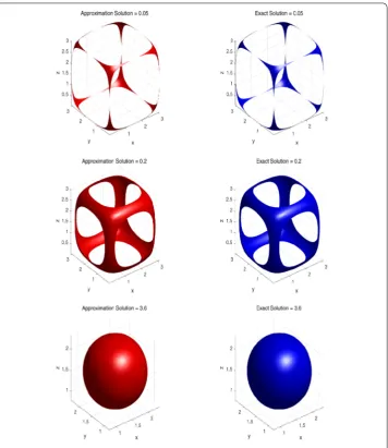
y=3₄π, the numerical and exact solutions are drawn at different times along thez-axis in Fig.2(c). Figure3 presents the graphs of isosurfaces of the numerical solution (red) and exact solution (blue) when three isovalues are assigned with meshh1=h2=h3=₅₀π,

Δβ=₂₀1, andτ =₂₀₀1 . It can be seen intuitively from all these figures that the numerical solution is highly consistent with the exact solution, which indicates the reliability of the algorithm (59)–(61) for the three-dimensional problem.

In Table5, taking the step sizesh1,h2,h3andΔβas fixed and small enough, then varying

the step sizes in time, the numerical errors in the discrete L2_{norm and the associated}

convergence orders are computed and illustrated. For scheme (59)–(61), the fixed step sizes are assigned ash1=h2=h3=π/100 andΔβ= 1/160. When scheme (62)–(64) is

employed, the step sizes in space and distributed order areh1=h2=h3=π/50 andΔβ=

1/10, respectively. This table shows numerical accuracy of difference schemes (59)–(61) and (62)–(64) in time, which agrees well with the theoretical results.

Figure 2Exact solutions (lines) and numerical solutions (symbols) att= 0.1 (red),t= 0.3 (magenta) and t= 0.5 (blue) by using scheme (59)–(61) (Example2)

in time, space and distributed order. This shows that the convergence orders of scheme (59)–(61) with respect to time, space and distributed order are approximately one, two and two, and that of scheme (62)–(64) are about one, two and four, respectively. The nu-merical results are in good agreement with the theoretical analysis, which demonstrates the effectiveness of the proposed methods for the three-dimensional problem.

Example3 We consider

2 1

5βC₀Dβtu(x,y,z,t)dβ

=∂

2_u(x,y,z,t)

∂x2 +

∂2u(x,y,z,t) ∂y2 +

∂2u(x,y,z,t) ∂z2

0 <t≤1, (x,y,z)∈Ω= (0, 1)×(0, 1)×(0, 1),

u(x,y,z,t) = 0, (x,y,z)∈∂Ω, 0≤t≤1,

Figure 3The graphs of isosurfaces for the approximation solution (red) and exact solution (blue) with different isovalues by scheme (59)–(61) (Example2)

Table 5 Errors and convergence orders of scheme (59)–(61) and scheme (62)–(64) in the temporal direction (Example2)

τ Scheme (59)–(61) Scheme (62)–(64)

eN

L2 Order CPU time eN L2 Order CPU time

1/10 0.1869 – 0.9506 s 0.1855 – 0.1057 s

1/20 0.0958 0.9642 2.0467 s 0.0944 0.9746 0.1882 s

1/40 0.0488 0.9731 4.8517 s 0.0474 0.9939 0.3908 s

1/80 0.0246 0.9882 12.9781 s 0.0232 1.0308 0.7970 s

1/160 0.0123 1.0000 39.2808 s 0.0108 1.1031 2.1005 s

Table 6 Errors and convergence orders of scheme (59)–(61) with an optimal step size ratio forτ,h1, h2,h3andΔβ(Example2)

τ h1=h2=h3 Δβ eN L2 Order eN L∞ Order CPU time

1/16 π/4 1/4 0.1717 – 0.0998 – 0.0285 s

1/64 π/8 1/8 0.0435 1.9808 0.0256 1.9629 0.0348 s

1/256 π/16 1/16 0.0108 2.0100 0.0064 2.0000 0.2327 s

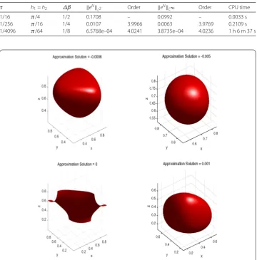
Table 7 Errors and convergence orders of scheme (62)–(64) with an optimal step size ratio forτ,h1, h2,h3andΔβ(Example2)

τ h1=h2 Δβ eN L2 Order eN L∞ Order CPU time

1/16 π/4 1/2 0.1708 – 0.0992 – 0.0033 s

1/256 π/16 1/4 0.0107 3.9966 0.0063 3.9769 0.2109 s

1/4096 π/64 1/8 6.5768e–04 4.0241 3.8735e–04 4.0236 1 h 6 m 37 s

Figure 4The graphs of isosurfaces for the approximate solution with different isovalues by scheme (59)–(61) (Example3)

In the current example, a three-dimensional distributed-order wave equation with a zero source term is considered. Figure4presents the graphs of isosurfaces of the numerical solution with meshh1=h2=h3=₁₀₀1 ,Δβ=₅₀1, andτ=₂₀₀1 at the final timeT= 1.

7 Conclusion

Acknowledgements

The authors would like to express their gratitude to the referees for their very helpful comments and suggestions on the manuscript.

Funding

This research was supported by the National Natural Science Foundation of China under grant 11471262.

Competing interests

The authors declare that they have no competing interests.

Authors’ contributions

JH carried out the numerical algorithms. JW conceived of the study and analyzed the theoretical results. YN helped to draft the manuscript. All the authors read and approved the final manuscript.

Author details

1_{Research Center for Computational Science, Northwestern Polytechnical University, Xi’an, China.}2_{College of Science,} Henan University of Technology, Zhengzhou, China.

Publisher’s Note

Springer Nature remains neutral with regard to jurisdictional claims in published maps and institutional affiliations.

Received: 24 January 2018 Accepted: 24 September 2018

References

1. Abbaszadeh, M., Dehghan, M.: An improved meshless method for solving two-dimensional distributed order time-fractional diffusion-wave equation with error estimate. Numer. Algorithms75(1), 173–211 (2016)

2. Atanackovic, T.M., Pilipovic, S., Zorica, D.: Time distributed-order diffusion-wave equation. I. Volterra-type equation. Proc. R. Soc. Lond., Ser. A, Math. Phys. Eng. Sci..465, 1869–1891 (2009)

3. Bhrawy, A.H., Zaky, M.A.: A method based on the Jacobi tau approximation for solving multi-term time-space fractional partial differential equations. J. Comput. Phys.281, 876–895 (2015)

4. Bhrawy, A.H., Zaky, M.A.: Numerical simulation of multi-dimensional distributed-order generalized Schrödinger equations. Nonlinear Dyn.89(2), 1415–1432 (2017)

5. Caputo, M.: Elasticità e dissipazione. Zanichelli, Bologna (1969)

6. Caputo, M.: Distributed order differential equations modelling dielectric induction and diffusion. Fract. Calc. Appl. Anal.4(4), 421–442 (2001)

7. Chechkin, A.V., Gorenflo, R., Sokolov, I.M. Gonchar, V.Y.: Distributed order time fractional diffusion equation. Fract. Calc. Appl. Anal.6(3), 259–280 (2003)

8. Chechkin, A.V., Klafter, J., Sokolov, I.M.: Fractional Fokker–Planck equation for ultraslow kinetics. Europhys. Lett.63(3), 326–332 (2003)

9. Dehghan, M., Abbaszadeh, M.: Element free Galerkin approach based on the reproducing kernel particle method for solving 2D fractional Tricomi-type equation with Robin boundary condition. Comput. Math. Appl.73(6), 1270–1285 (2017)

10. Diethelm, K., Ford, N.J.: Numerical analysis for distributed-order differential equations. J. Comput. Appl. Math.225(1), 96–104 (2009)

11. Eab, C., Lim, S.: Fractional Langevin equations of distributed order. Phys. Rev. E83(3), 031136 (2011)

12. Ford, N.J., Morgado, M.L., Rebelo, M.: An implicit finite difference approximation for the solution of the diffusion equation with distributed order in time. Electron. Trans. Numer. Anal.44, 289–305 (2015)

13. Gao, G., Sun, H., Sun, Z.: Some high-order difference schemes for the distributed-order differential equations. J. Comput. Phys.298, 337–359 (2015)

14. Gao, G., Sun, Z.: Two alternating direction implicit difference schemes with the extrapolation method for the two-dimensional distributed-order differential equations. Comput. Math. Appl.69(9), 926–948 (2015) 15. Gao, G., Sun, Z.: Two alternating direction implicit difference schemes for solving the two-dimensional time

distributed-order wave equations. J. Sci. Comput.69(2), 506–531 (2016)

16. Gao, G., Sun, Z.: Two alternating direction implicit difference schemes for two-dimensional distributed-order fractional diffusion equations. J. Sci. Comput.66(3), 1281–1312 (2016)

17. Gao, G., Sun, Z.: Two unconditionally stable and convergent difference schemes with the extrapolation method for the one-dimensional distributed-order differential equations. Numer. Methods Partial Differ. Equ.32(2), 591–615 (2016)

18. Gorenflo, R., Luchko, Y., Stojanovi´c, M.: Fundamental solution of a distributed order time-fractional diffusion-wave equation as probability density. Fract. Calc. Appl. Anal.16(2), 297–316 (2013)

19. Hartley, T.T., Lorenzo, C.F.: Fractional system identification: an approach using continuous order-distributions. NASA (1999)

20. Jiao, Z., Chen, Y., Podlubny, I.: Distributed-Order Dynamic Systems: Stability, Simulation, Applications and Perspectives. Springer Briefs in Electrical and Computer Engineering, pp. 90–97. Springer, London (2012)

21. Katsikadelis, J.T.: Numerical solution of distributed order fractional differential equations. J. Comput. Phys.259, 11–22 (2014)

22. Kochubei, A.N.: Distributed order calculus and equations of ultraslow diffusion. J. Math. Anal. Appl.340(1), 252–281 (2008)

24. Morgado, M.L., Rebelo, M.: Numerical approximation of distributed order reaction–diffusion equations. J. Comput. Appl. Math.275, 216–227 (2015)

25. Podlubny, I., Skovranek, T., Jara, B.M.V., Petras, I., Verbitsky, V., Chen, Y.: Matrix approach to discrete fractional calculus III: non-equidistant grids, variable step length and distributed orders. Philos. Trans. R. Soc. Lond. A371(1990), 20120153 (2013)

26. Quarteroni, A., Valli, A.: Numerical Approximation of Partial Differential Equations. Springer Series in Computational Mathematics, vol. 23. Springer, Berlin (2008)

27. Rida, S., El-Sayed, A., Arafa, A.: On the solutions of time-fractional reaction–diffusion equations. Commun. Nonlinear Sci. Numer. Simul.15(12), 3847–3854 (2010)

28. Samarskii, A., Andreev, V.: Difference Methods for Elliptic Equations. Nauka, Moscow (1976)

29. Sinai, Y.G.: The limiting behavior of a one-dimensional random walk in a random medium. Theory Probab. Appl.27(2), 256–268 (1983)

30. Sun, Z.: The Method of Order Reduction and Its Application to the Numerical Solutions of Partial Differential Equations. Science Press, Beijing (2009)

31. Wazwaz, A.M., Gorguis, A.: An analytic study of Fisher’s equation by using Adomian decomposition method. Appl. Math. Comput.154(3), 609–620 (2004)

32. Ye, H., Liu, F., Anh, V.: Compact difference scheme for distributed-order time-fractional diffusion-wave equation on bounded domains. J. Comput. Phys.298, 652–660 (2015)

33. Zaky, M.A.: A Legendre spectral quadrature tau method for the multi-term time-fractional diffusion equations. Comput. Appl. Math.37(3), 3525–3538 (2018)

34. Zaky, M.A.: A Legendre collocation method for distributed-order fractional optimal control problems. Nonlinear Dyn. 91(4), 2667–2681 (2018)