R E S E A R C H
Open Access
The computation of the viability kernel for
switched systems
Jianfeng Lv
1,2and Yan Gao
1**Correspondence: [email protected]
1School of Management, University of Shanghai for Science and Technology, Shanghai, China Full list of author information is available at the end of the article
Abstract
The computation of the viability kernel provides the guarantee for the security evolution of the systems. In this paper, we focus on the computation of the viability kernel for discrete-time and continuous-time switched systems. A connection between the backward reachable set and the viability kernel for switched systems is established. The methods of computing the viability kernel for switched systems are constructed by using this connection. First, a method of computing the viability kernel for discrete-time switched systems is proposed. Then, taking into account the special structure of switched linear systems, a simple algorithm that is easy to implement is developed. Moreover, the methods of dealing with the discrete systems are extended to the continuous systems, and the algorithms of computing the viability kernel for continuous-time switched systems and switched linear systems are proposed. Finally, examples are listed to illustrate the effectiveness of the main results.
Keywords: Switched systems; Control; Viability kernel; Reachable set
1 Introduction
The problem of viability [1] concerns the dynamic evolutions governed by complex sys-tems under uncertainty that are found in many domains involving living beings, from bi-ological evolution to economics [2], from environmental sciences to financial markets [3,
4], from control theory to cognitive sciences [5–7]. It aims at controlling dynamical sys-tems with the goal to maintain the state of the syssys-tems inside a given set which we called the constraint set or safe region. Determining the viability on a constraint set has been researched in the references [8–12]. When faced with the constraint set that is not viable, one would like to establish a subset of the constraint set that is viable. This subset is said to be the viability kernel (or the maximal invariant set).
Computation of the viability kernel for dynamical systems is a fundamental problem in the viability theory. It has traditionally been computed using the viability kernel algorithm [13] and level set approach [14]. However, these methods require gridding the state space, and hence their time and memory complexity grow exponentially with the state dimen-sion. Thus, these methods are feasible only for dynamical systems with low dimendimen-sion. To overcome this limitation, researchers considered the same problem by using dynamic pro-gramming [15] and support vector machines [16]. Recently, Maidens in [17] proposed an algorithm of computing the viability kernel by using backward reachable set for dynamical
systems. Since there are some efficient techniques for computing the maximal reachable set in [18,19], these methods can be used to compute the viability kernel [17].
Switched systems, which consist of two or more subsystems and a switching signal or-chestrating switching between these subsystems, have attracted a growing interest in re-cent years. The viability kernel for switched systems has been largely studied, and several results have been reported in [20–28]. Aubin and Lygeros introduced a notion of hybrid strategy and proved convergence of the iterative algorithm by using non-smooth analysis tools in [23]. Margellos and Lygeros proposed a method of computing the viable set for hy-brid systems [24] in the context of optimal control, and a complete characterization of the computation of the viable set was provided based on dynamic programming. Haimovich et al. in [25] also developed a method of computing the invariant set for continuous-time switched linear systems with disturbances and arbitrary switching. Abate and Prandini in [26] studied probabilistic reachability over a finite horizon for a class of discrete time stochastic hybrid systems. Lygeros et al. in [27] presented some simple properties of the invariant sets for hybrid automata, and the invariance principle was extended to hybrid automata. By establishing a link between reachability, viability, and invariance problems and viscosity solutions of a special form of the Hamilton–Jacobi equation, the numeri-cal algorithm developed for the approximation of viscosity solutions to partial differential equations was extended to viability and invariance computation in [28].
It should be noted that all the methods in [23–25,28] have certain limitations when they are executed. The first is that many conditions must be satisfied in the implementation of the algorithms. In order to guarantee the convergence of these algorithms, we need to compute the maximal fixed point of a monotone operator on a complete lattice of closed sets in [24] and determine the transformation matrix satisfying certain properties in [25]. The given set must be open and the partial differential equation must have a special form (standard Hamilton–Jacobi form, continuity of the Hamiltonian, and simple boundary conditions) in [28]. Thus, the convergence conditions are too strong. Moreover, because of the large amount of computation and considerable time consumption, the implementation of the algorithms is difficult. To overcome these limitations, we restrict our attention to switched linear systems. Since they have a special structure, the limitations of [23–25,28] can be solved effectively. Thus, we try to design a simple method of computing the viability kernel for switched linear systems.
The organization of the paper is as follows. In Sect.2we introduce some necessary pre-liminaries. Section3discusses the computation of the viability kernel for discrete-time switched systems and develops a simple algorithm for discrete-time switched linear sys-tems. Furthermore, we compute the viability kernel for continuous-time switched systems and propose an algorithm for switched linear systems in Sect.4. We provide several ex-amples in Sect.5.
2 Preliminaries
Consider the following switched system: ⎧
⎨ ⎩
L(x(t)) =fσ(t)(x(t),u(t)),
u(t)∈U, (2.1)
where the statex∈Rn, the controlu∈U,U⊂Rm, the functionf
σ : Rn×U→Rn, and the
or discrete (T = [0,τ]∩Z+). If 0 <τ <∞, problem (2.1) is said to have a finite
hori-zon; ifτ =∞, it is said to have an infinite horizon.L(·) denotes the derivative operator for continuous-time switched systems or the difference operator for the case of discrete-time.σ(t) : [t0, +∞)→is a switching signal that is a piecewise constant function of time
tand takes values at the sampling times in a finite set={1, . . . ,N}, whereN> 1 is the number of subsystems.σ(t) =i(i∈) denotes that the subsystemfiis activated. We
as-sume that the functionsfi(i∈) are sufficiently smooth to guarantee the existence and
uniqueness of solutions to the corresponding initial value problems. We refer to the se-quencet0,t1, . . . ,tsas a switching time sequence, and the sequenceσ(t0),σ(t1), . . . ,σ(ts) as
a switching index sequence. It is clear that these two sequences can uniquely determine the switching path, and vice versa.
In order to discuss the method of computing the viability kernel conveniently, we present some important features of switched systems. Switched systems are dynamical systems that consist of a finite number of subsystems and a logical rule that orchestrates switching between these subsystems. Therefore, one of the features of switched systems is multi-subsystem. In addition, switched systems could not be guaranteed to be stable even if all subsystems are stable. Switching rule may be designed to stabilize switched systems even if all subsystems are unstable. According to the discussion above, the computation of the viability kernel is affected by the switching rules and subsystems.
We start with some notions, which will be used later on.
Definition 1 LetK⊂Rn. The viability kernel of system (2.1) on the setKover the time
horizonTis defined as follows:
ViabT(K) =
x0∈K|∃u0:T→U,∀t∈T,x(t)∈K
. (2.2)
Obviously, ViabT(K) contains all initial states inK for which there exists an input such
that the trajectories starting from those states remain withinKfor all timet∈T.
Definition 2 The backward reachable set fromKat timetis defined as follows:
Reacht(K) =
x0∈Rn|∃u0∈U,x(t)∈K
. (2.3)
In fact, the backward reachable set contains all initial states for which there exists an input such that the trajectories emanating from those states reachKexactly at timet.
3 The viability kernel of discrete-time switched systems
In this section, we establish a connection between the viability kernel and the reachable set for discrete-time switched systems. Then, we discuss algorithms of computing the viability kernel in terms of the reachable set.
3.1 Discrete-time switched systems
We consider the discrete-time switched systems as follows:
x(t+ 1) =fσ(t)
x(t),u(t), (3.1)
where the timet∈T = [0,τ]∩Z+and switching signalσ∈={1, . . . ,N}. We next discuss
how to compute the viability kernel on the given regionKby using the maximal reachable set. As we know, the viability kernel for discrete-time dynamical systems can be computed using Saint-Pierre’s viability kernel algorithm (see [13]). In the light of Saint-Pierre’s via-bility kernel algorithm, we give an iterative formula of the viavia-bility kernelKn+1:= ViabT(K)
for system (3.1) on the finite horizonT = [0,n+ 1]∩Z+:
⎧ ⎨ ⎩
K0=K,
Kn+1={x∈Kn|Kn∩F(x)=∅},
(3.2)
whereF(x) ={fσ(x,u)|u∈U,σ∈}. We replace the finite horizon viability kernelKnin
(3.2) by the backward reachable set. Then we obtain the following theorem.
Theorem 1 The viability kernel over a finite horizon T = [0,n+ 1]∩Z+for system(3.1)
on the set K can be computed by the following recursive formula: ⎧
⎨ ⎩
K0=K,
Kn+1=K0∩Reach1(Kn).
(3.3)
Proof System (3.1) can be written as the difference inclusion
x(t+ 1)∈Fx(t), t= 0, 1, . . . ,n,
whereF(x) ={fσ(x,u)|u∈U,σ∈}. First, we prove the following formula:
ViabT(K) =Kn∩Reach1(Kn). (3.4)
By the definition of ViabT(K) and (3.2), we have x∈Kn andKn∩F(x)=∅ when x∈
ViabT(K). It means that there existsysuch thaty∈Knandy∈F(x). Then there existu∈U
andσ∈such thaty=fσ(x,u). Thus, we haveu∈Uandσ∈such thatfσ(x,u)∈Kn.
According to (2.3) andx∈Kn, we havex∈Reach1(Kn). Moreover, we obtain that x∈
Kn∩Reach1(Kn). Similarly, we concluded thatx∈ViabT(K) formx∈Kn∩Reach1(Kn).
This means that
Therefore, we only need to prove that
Kn∩Reach1(Kn) =K0∩Reach1(Kn).
According to (3.4), we have
Kn+1=Kn∩Reach1(Kn),
which implies that
Kn+1⊆Kn⊆ · · · ⊆K1⊆K0
and
Reach1(Kn)⊆Reach1(Kn–1)⊆ · · · ⊆Reach1(K1)⊆Reach1(K0).
Thus, we get
Kn+1=K0∩Reach1(K0)∩Reach1(K1)∩ · · · ∩Reach1(Kn)
=K0∩Reach1(Kn).
This completes the proof of the theorem.
Theorem 1 gives us a method of constructing a finite horizon viability kernel for discrete-time switched systems (3.1). In (3.3), we compute the viability kernel by K0∩
Reach1(Kn) instead ofKn∩Reach1(Kn), though they are equivalent when the reachable
set and the operation of intersections can be computed exactly. In fact,K0is simpler and
more precise in implementation thanKn. Thus, we construct the viability kernel by
recur-sive formula (3.3). In what follows, the key problem we need to solve is the computation of the reachable set for switched systems.
The computation of the reachable set for dynamical systems is given in [17]. The reach-able states of dynamical systems are affected by the system and the control input. Since switched systems have many subsystems, the trajectories of switched systems are re-stricted by multiple subsystems and the reachability is also affected by the switching rules. Different switching rules lead to different reachable states. Thus, the computation of the reachable set for switched systems is more complex than for dynamical systems. We as-sume that the switching rules are arbitrary switches. In this case, we need to compute the possible reachable region for every subsystem. Then the reachable set for switched systems is obtained by taking the union of all the reachable regions.
We next illustrate the computation process of the reachable setReach1(K) for system
(3.1) on the setKover a unit time step in detail. First, we need to compute the reachable set ofKfor every subsystemfσ(x,u),σ∈, and the obtained set is denoted byReachσ1(K),
σ∈. So we getNreachable sets. Then the setReach1(K) can be got by intersecting these Nreachable sets
Reach1(K) =
N
i=1
Algorithm 1The viability kernel of discrete-time switched systems LetK0←K
l←0 whilel≤ndo
ifKl=∅then
Kn← ∅
break endif
ifKl=Kl–1then
Kn←Kl
break endif
L←Ni=1Reachi1(Kl)
Kl+1←K0∩L
l←l+ 1 end while returnKn
The amount of the computation is proportional to the number of the subsystems. When the number of the subsystems is higher, the amount of the computation is greater.
According to Theorem1, an algorithm of computing the viability kernel for system (3.1) over a finite horizonT = [0,n]∩Z+is proposed (see Algorithm1).
Algorithm1transforms the computation of the viability kernel on a finite horizon into the computation of the reachable set for finite times. The main advantages of Algorithm1
are as follows: The first is that the key problem in the iteration is the computation of the reachable set. Many researchers are devoted to the computation of the reachable set for dynamical systems, and many methods of computing the reachable set are proposed. Since the methods of computing the reachable set for dynamical systems are extended to switched systems, Algorithm1is available in practice. The second is that the set obtained from Algorithm1is the exact viability kernel of system (3.1) on the given set.
3.2 Discrete-time switched linear systems
Algorithm1can be applied to switched nonlinear systems in theory. However, the com-putation process of nonlinear systems is rather complex and troublesome. The complexity of computing the reachable set lies in the part of nonlinear continuous evolution. Thus, we consider the viability kernel for switched linear systems. Due to the special structure of linear systems, which have some special properties, we discuss a simple algorithm of computing the viability kernel for switched linear systems. In this subsection, we consider the following discrete-time switched linear systems:
x(t+ 1) =Aσx(t) +Bσu(t), (3.5)
where the statex∈Rn, the timet∈T = [0,n]∩Z
+, the control inputu∈U,Uis a
com-pact set, and switching signalσ takes values in a finite set={1, . . . ,N}. Aσ ∈Rn×nis
an invertible matrix andBσ ∈Rn×m. As we know, any region can be approximated by a
develop an efficient algorithm of computing the backward reachable set for system (3.5) on the constraint setK.
Due to the special structure of linear systems, (3.5) can be rewritten as
x(t+ 1) =Aσx(t) –v(t),
wherev(t)∈Vσ ={–Bσu|u∈U}. In the case of discrete-time, the backward reachable set
of subsystemA1over a unit time step is computed as follows:
Reach(K) =A–11 (K⊕V1). (3.6)
The operator⊕means the Minkowski sum of two sets.A–1
1 (·) denotes the preimage of a
set under the mapA1. Similarly, the backward reachable set of subsystemAl(l= 2, . . . ,N)
over a unit time step is obtained by
Reach(K) =A–1l (K⊕Vl). (3.7)
According to the discussion above, we get the reachable set of system (3.5) on the setKas follows:
Reach(K) =A–11 (K⊕V1)∪ · · · ∪A–1N(K⊕VN)
=
N
i=1
A–1i (K⊕Vi), (3.8)
whereVi={–Biu|u∈U},i∈.
Formula (3.8) gives us a method of computing the reachable set in the case of linear systems. In this method, the computation of the reachable set is transformed into several operations on the sets. As long as the matrices of all the subsystems are invertible, the reachable set can be expressed by (3.8). It is true for linear systems, but not for nonlinear systems. From (3.8), the computation of the reachable set involves the operations per-formed on sets including Minkowski sum, linear transformation, and union. In addition, it is easy to see that the operation of intersection on sets is required in the computation of the viability kernel. In the following, we illustrate the processes of these operations per-formed on sets of polytopes.
Let
K=x∈Rn|H1x≤b1
,
V=x∈Rn|H2x≤b2
.
(3.9)
We can compute the preimage ofKunder the linear transformationAias follows:
A–1i K=x∈Rn|H1A–1i x≤b1
The intersection and union ofKandVcan also be easily computed, respectively.
However, the Minkowski sum is difficult to compute using the representations as (3.9). We need to convert them to another form. In fact, a polytope can also be expressed by its vertices (see [29])
In fact, (3.10) is equivalent to (3.9). This is a well-studied problem, and many algorithms have been proposed to solve it. Then the Minkowski sum ofKandV is given as follows [29]:
K⊕V= cowi+vj|i= 1, . . . ,m;j= 1, . . . ,n
.
Moreover, the setK⊕Vis also a polytope.
According to the discussion above, we can give a method of computing the reachable set on the polyhedral constraint set and the polyhedral input set. Applying (3.8) to Algo-rithm1, we obtain an algorithm of computing the viability kernel for system (3.5) on the finite horizonT(see Algorithm2).
It should be noted that the formula of computing the reachable set can be expressed by the operations on the constraint set and the control input set. Moreover, we get the via-bility kernel by implementing the operations on sets including intersection, union, linear transformation, and Minkowski sum. These operations are easy to implement when both the constraint set and the control input set are polytopes. Therefore, the algorithm has a small amount of computation.
3.3 Analysis of the algorithms
We next give some basic properties of Algorithms1,2.
Theorem 2 If Algorithm 1 terminates with l < n and Kl =∅, then Viab[0,n]∩Z+(K) =
∅ and Viab[0,∞)∩Z+(K) =∅. If Algorithm 1 terminates with l <n and Kl =Kl–1, then
Viab[0,n]∩Z+(K) =KlandViab[0,∞)∩Z+(K) =Kl.
Proof The viability kernel over a finite horizonT= [0,n]∩Z+is empty when Algorithm1
Algorithm 2The viability kernel of discrete-time switched linear systems LetK0←K
l←0 whilel≤ndo
ifKl=∅then
Kn← ∅
break endif
ifKl=Kl–1then
Kn←Kl
break endif
L←Ni=1A–1
i (Kl⊕Vi)
Kl+1←K0∩L
l←l+ 1 end while returnKn
the given regionKwill leaveKat thekth (k≥l) step of the algorithm. Thus, the viability kernel over an infinite horizon is also empty, that is, Viab[0,∞)∩Z+(K) =∅.
If Algorithm1terminates withl<nandKl=Kl–1, according to Theorem1, the viability
kernel over a finite horizonT is Viab[0,n]∩Z+(K) =Kl. In fact, at thekth (k>l) step of the
algorithm, we have
Kk=Kl. (3.11)
Equation (3.11) still holds whenktends to infinity. This tells us that Viab[0,∞)∩Z+(K) =Kl.
This completes the proof of the theorem.
Algorithm2is a special case of Algorithm1, thus it has the same conclusion.
4 The viability kernel of continuous-time switched systems
In this section, we discuss the computation of the viability kernel for continuous-time switched systems. By discretizing continuous-time systems, two efficient algorithms of approximating the viability kernel are developed by using the result of Sect.3.
4.1 Continuous-time switched systems Consider the following system:
˙
x(t) =fσ(t)
x(t),u(t), (4.1)
where the functionfσ is bounded byM> 0 on the constraint setK⊆Rn. It means that for
allx∈Kandu∈U, we havefσ(x(t),u(t)) ≤M,σ∈. We define a distance of a point
x∈Rnfrom a nonempty setS⊂Rnas follows:
dS(x) =inf
In the following, we compute an under-approximation of the viability kernel for system (4.1) on the finite horizonT = [0,τ]. Given a discretization time stepδ, define an under-approximation of the viability constraint set
Kδ=
x∈K|dKc(x)≥δM. (4.3)
Kδ approximates toKby the distanceδMbecause we only consider the state at discrete
timestk=kδ. For any interval [tk,tk+1], the solution of (4.1) does not leaveKat any time
t∈[tk,tk+1]. In fact, a solutionx(t) of (4.1) can travel a distance of at mostδMfrom its
initial statex(tk).
x(tk) –x(t)≤ t tk
x(˙τ)dτ ≤M(t–tk)≤δM.
Thus, we define the recursive formula as follows: ⎧
⎨ ⎩
K0(δ) =Kδ,
Kn+1(δ) =K0(δ)∩Reachδ(Kn(δ)).
(4.4)
At each step, we compute the set of states from whichKn(δ) is reachable, and then intersect
this set with K0(δ). Each computed setKn(δ) is an approximation of the finite horizon
viability kernel Viab[0,τ](K) forτ=nδ.
Theorem 3 Assume that fσ is bounded by M> 0on the set K for allσ∈.For any time
stepδ,the set{Kn(δ)}produced by(4.4)satisfies
Kn(δ)⊆Viab[0,nδ](K). (4.5)
Proof In order to obtain the reachable set ofKn(δ) for system (4.1), we first compute the
reachable set ofKn(δ) for every subsystemfσ(x,u),σ∈ {1, . . . ,N}. Thus, we getNreachable
sets. So the reachable setReachδ(Kn(δ)) can be obtained by intersecting theseNreachable
sets. The rest of the proof is similar to that of Theorem 2 in [17]. This completes the proof
of the theorem.
Theorem 4 Suppose that fσ is bounded by M> 0on the set K for allσ∈.For any time
stepδ,the set{Kn(δ)}produced by(4.4)satisfies
Viab[0,τ]
int(K)⊆
n∈N
Kn(δ)⊆Viab[0,τ](K). (4.6)
Proof According to (4.5) and Theorem 3 in [17], the set{Kn(δ)}produced by (4.4) satisfies
(4.6). This completes the proof of the theorem.
According to (4.5) and (4.6), the setKn(δ) produced by (4.4) is an under-approximation
of the finite horizon viability kernel Viab[0,τ](K) forτ =nδ. Then we get an algorithm of
Algorithm 3The viability kernel of continuous-time switched systems Chooseδ> 0
n←τ δ
K0←Kδ
l←0
whilel≤ndo ifKl=∅then
Kn← ∅
break endif
ifKl=Kl–1then
Kn←Kl
break endif
L←Reach[0,δn](Kl)
Kl+1←K0∩L
l←l+ 1 end while returnKn
Algorithm3gives us a method of computing the viability kernel over a finite horizon for continuous-time switched systems. The main iterative process of the algorithm is as follows. First, we define an under-approximationK0(δ) of the given set and compute the
set of backward reachable states fromK0(δ). Next, we intersect the backward reachable
set withK0(δ) to getK1(δ) and compute the reachable set fromK1(δ). Then, we intersect
the reachable set withK0(δ) to get a new setK2(δ). By repeating this process, we eventually
reach an under-approximation of the viability kernel.
4.2 Continuous-time switched linear systems
Since linear systems have special structure and some special properties, it is more con-venient to compute the reachable set. Thus, we consider a simple algorithm of approxi-mating the viability kernel for switched linear systems. Let us restrict our attention to the following system:
˙
x(t) =Aσx(t) +Bσu(t), (4.7)
where the statex∈Rn, the timet∈T = [0,τ]∩R
+, the control inputu∈U,Uis a compact
and convex set, and switching signalσtakes values in a finite set={1, . . . ,N}.Aσ ∈Rn×n
is an invertible matrix and bounded byMandBσ∈Rn×m. Before computing the backward
reachable set of system (4.7) on the constraint setK, we introduce a notion of Hausdorff distance.
Definition 3 LetX,Y be nonempty compact convex subsets of Rn. The Hausdorff
dis-tance ofXandYis defined as follows:
dH(X,Y) =max
sup
x∈X
inf
y∈Yx–y,supy∈Yxinf∈Xx–y
We next compute an approximation of the reachable set by discretizing system (4.7). By choosing a time stepδ, the number of time steps isn=τ
δ. Suppose that the control
u(t) =u(t˜ i) is constant over the time interval [ti,ti+1],i= 0, 1, . . . ,n– 1. We discretize system
(4.7) by using Eulerian method, then we have
⎧
Applying Theorem 1 of [30] to system (4.7) and the corresponding discretization system (4.9), we obtain the following result.
Theorem 5 Suppose thatReach[0,δn](Kl)andReach˜ [0,δn](Kl)are the backward reachable
sets of systems(4.7)and(4.9)on the set Klover the time interval[tl,tl+1],respectively.Then
there exists a constant C such that
dH
Reach[0,δn](Kl),Reach˜ [0,δn](Kl)
≤Cδ, (4.10)
whereδis a discretization time step.
Proof The conclusion can be established by following Theorem 1 in [30]. This completes
the proof of the theorem.
Theorem 5 shows us that the Hausdorff distance between the reachable sets Reach[0,δn](Kl) andReach˜ [0,δn](Kl) has an upper bound, and the distance is proportional
to the size ofδ. Moreover, whenδis smaller, the upper bound of the associated Hausdorff distance is smaller. Theorem5provides us a theoretical basis for usingReach˜ [0,δn](Kl)
ap-proximating toReach[0,δn](Kl), that is, we can obtain an approximation of the reachable
set for a continuous-time system by computing the reachable set for the corresponding discretization system. Thus, we only need to compute the reachable set for system (4.9), which is equivalent to the following system:
˜
x(t+ 1) = (I+δAσ)x(t) +˜ δBσu(t).˜ (4.11)
Iis an identity matrix. SettingVσ = –δBσU={–δBσu(t)˜ |˜u(t)∈U}, the reachable set over
a single time step can be computed as follows:
Algorithm 4The viability kernel of continuous-time switched linear systems
Based on Algorithm3and (4.12), we propose an algorithm of computing an approxima-tion of the viability kernel for system (4.7) (see Algorithm4).
Algorithm4is the development of Algorithm3in the case of linear systems. The compu-tation of the reachable set has been simplified. Moreover, an approximation of the viability kernel can be obtained by computing the viability kernel of the corresponding discretiza-tion system. The approximadiscretiza-tion error can be made arbitrarily small by choosingδsmall enough.
Algorithms3and4have the same properties as listed in Theorem2. The proof is similar to that of Theorem2, and we do not illustrate it in detail.
5 Illustrative examples
5.1 Example 1
Consider the following discrete-time switched linear system:
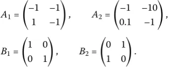
A1=
assume that the control input set
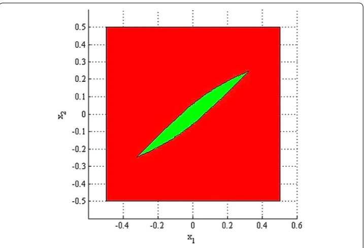
Figure 1Viability constraint (5.3) (red) and the corresponding viability kernel (green) for (5.1) by using Algorithm2
We next compute the viability kernel for system (5.1) on the state constraint set (5.3) with a horizon of 40 steps. The viability kernel can be obtained by using Algorithm2, the result shows in Fig.1.
Figure1shows us that the red region is the viability constraint set, and the green region is the viability kernel for system (5.1).
5.2 Example 2
Consider the following continuous-time switched linear system:
A1=
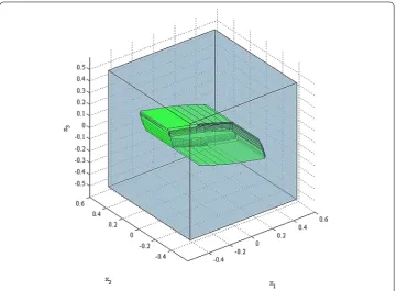
The control input set and the state constraint set are given by (5.2) and (5.3), respec-tively. We compute the viability kernel of system (5.4) on the region (5.3) with the time horizon [0, 4]. Choosing the time stepδ= 0.1, we discretize system (5.4). Then we obtain an approximation of the viability kernel by using Algorithm4. The result shows in Fig.2.
5.3 Example 3
Consider the following discrete-time switched linear system:
Figure 2Viability constraint (5.3) (red) and the corresponding viability kernel (green) for (5.4) by using Algorithm4
whereI is an identity matrix, the statex∈R3, the timet∈T = [0,n]∩R
+, the control
inputu∈U⊂R3. We assume that the control input set
U=u= (u1,u2,u3)T|–0.03≤ui≤0.03,i= 1, 2, 3
, (5.6)
and the state constraint set
K=x= (x1,x2,x3)T|–0.5≤xi≤0.5,i= 1, 2, 3
. (5.7)
We next compute the viability kernel for system (5.5) on the state constraint set (5.7) with a horizon of 10 steps. The viability kernel can be obtained by using Algorithm2, the result shows in Fig.3.
6 Conclusions
Figure 3Viability constraint (5.7) (grey) and the corresponding viability kernel (green) for (5.5) by using Algorithm2
Acknowledgements
This work is supported by the National Natural Science Foundation of China under Grant No.11171221, Doctoral Program Foundation of Institutions of Higher Education of China under Grant No.20123120110004.
Funding
This work is supported by the National Natural Science Foundation of China under Grant No.11171221, Doctoral Program Foundation of Institutions of Higher Education of China under Grant No.20123120110004.
Competing interests
The authors declare that they have no competing interests.
Authors’ contributions
All authors contributed equally to the writing of this paper. All authors read and approved the final manuscript.
Author details
1School of Management, University of Shanghai for Science and Technology, Shanghai, China.2School of Science, Inner
Mongolia University of Science and Technology, Baotou, China.
Publisher’s Note
Springer Nature remains neutral with regard to jurisdictional claims in published maps and institutional affiliations.
Received: 30 March 2018 Accepted: 13 August 2018 References
1. Aubin, J.P.: Viability Theory. Springer, Berlin (2011)
2. Béné, C., Doyen, L., Gabay, D.: A viability analysis for a bio-economic model. Ecol. Econ.36(3), 385–396 (2001) 3. Mullon, C., Cury, P., Shannon, L.: Viability model of trophic interactions in marine ecosystems. Nat. Resour. Model.
17(1), 71–102 (2004)
4. Sanogo, C., Raïssi, N., Miled, S.B., et al.: A viability analysis of fishery controlled by investment rate. Acta Biotheor.61(3), 341–352 (2013)
5. Liu, L., Gao, Y., Wu, Y.P.: Speed optimization control for wheeled robot navigation with obstacle avoidance based on viability theory. Automatika57(2), 428–440 (2017)
6. Spiteri, R.J., Pai, D.K., Ascher, U.M.: Programming and control of robots by means of differential algebraic inequalities. IEEE Trans. Robot. Autom.16(2), 135–145 (2000)
8. Chen, Z., Gao, Y.: Determining the viable unbounded polyhedron under linear control systems. Asian J. Control16(5), 1561–1567 (2014)
9. Lou, Z.E., Gao, Y.: The exponential stability for a class of hybrid systems. Asian J. Control15(2), 624–629 (2013) 10. Dong, X.X., Zhao, J.: Incremental passivity and output tracking of switched nonlinear systems. Int. J. Control85(10),
1477–1485 (2012)
11. Gao, Y.: Viability criteria for differential inclusions. J. Syst. Sci. Complex.24(5), 825–834 (2011)
12. Lv, J.F., Gao, Y., Zhao, N.: Viability criteria for a switched system on bounded polyhedron. Asian J. Control (2017, in press).https://doi.org/10.1002/asjc.1719
13. Saint-Pierre, P.: Approximation of viability kernel. Appl. Math. Optim.29(2), 187–209 (1994)
14. Mitchell, I.M., Bayen, A.M., Tomlin, C.J.: A time-dependent Hamilton–Jacobi formulation of reachable sets for continuous dynamic games. IEEE Trans. Autom. Control50(7), 947–957 (2005)
15. Coquelin, P.A., Martin, S., Munos, R.: A dynamic programming approach to viability problems. In: IEEE International Symposium on Approximate Dynamic Programming and Reinforcement Learning, pp. 178–184 (2007)
16. Deffuant, G., Chapel, L., Martin, S.: Approximating viability kernels with support vector machines. IEEE Trans. Autom. Control52(5), 933–937 (2007)
17. Maidens, J.N., Kaynama, S., Mitchell, I.M., Oishi, M.M.K.: Lagrangian methods for approximating the viability kernel in high-dimensional systems. Automatica49, 2017–2029 (2013)
18. Kaynama, S., Mitchell, I.M., Oishi, M., et al.: Scalable safety-preserving robust control synthesis for continuous-time linear systems. IEEE Trans. Autom. Control60(11), 3065–3070 (2015)
19. Maidens, J., Arcak, M.: Reachability analysis of nonlinear systems using matrix measures. IEEE Trans. Autom. Control 60(1), 265–270 (2015)
20. Fribourg, L., Goubault, E., Putot, S., et al.: A topological method for finding invariant sets of switched systems. In: Proceedings of the 19th International Conference on Hybrid Systems: Computation and Control, pp. 61–70. ACM, New York (2016)
21. Riedinger, P., Sigalotti, M., Daafouz, J.: On the algebraic characterization of invariant sets of switched linear systems. Automatica46(6), 1047–1052 (2010)
22. Han, Y., Gao, Y.: The calculation of discriminating kernel based on viability kernel and reachability. Adv. Differ. Equ. 2017, 370 (2017)
23. Aubin, J.P., Lygeros, J., Quincampoix, M., et al.: Impulse differential inclusions: a viability approach to hybrid systems. IEEE Trans. Autom. Control47(1), 2–20 (2002)
24. Margellos, K., Lygeros, J.: Viable set computation for hybrid systems. Nonlinear Anal. Hybrid Syst.10, 45–62 (2013) 25. Haimovich, H., Seron, M.M.: Componentwise ultimate bound and invariant set computation for switched linear
systems. Automatica46(11), 1897–1901 (2010)
26. Abate, A., Prandini, M., Lygeros, J., et al.: Probabilistic reachability and safety for controlled discrete time stochastic hybrid systems. Automatica44(11), 2724–2734 (2008)
27. Lygeros, J., Johansson, K.H., Simic, S.N., et al.: Dynamical properties of hybrid automata. IEEE Trans. Autom. Control 48(1), 2–17 (2003)
28. Lygeros, J.: On reachability and minimum cost optimal control. Automatica40(6), 917–927 (2004)
29. Kvasnica, M., Grieder, P., Baoti´c, M., et al.: Multi-parametric toolbox (MPT). In: Hybrid Systems: Computation and Control, pp. 448–462 (2004)