circuits using geometric algebra and evolutionary
algorithms
Francisco G. Montoya1* , Alfredo Alcayde1, Francisco M. Arrabal-Campos1, Raul Baños1
1 Dept. of Engineering, University of Almeria, Spain; [email protected] [email protected] [email protected] and
* Correspondence: [email protected]; Tel.: +34 950 214501
Abstract:Non-linear loads in circuits cause the appearance of harmonic disturbances both in voltage and current. In order to minimize the effects of these disturbances and, therefore, to control over the flow of electricity between the source and the load, they are often used passive or active filters. Nevertheless, determining the type of filter and the characteristics of their elements is not a trivial task. In fact, the development of algorithms for calculating the parameters of filters is still an open question. This paper analyzes the use of genetic algorithms to maximize the power factor compensation in non-sinusoidal circuits using passive filters, while concepts of geometric algebra theory are used to represent the flow of power in the circuits. According to the results obtained in different case studies, it can be concluded that the genetic algorithm obtain high quality solutions that could be generalized to similar problems of any dimension.
Keywords: Power factor compensation; non-sinusoidal circuits; geometric algebra; evolutionary algorithms.
1. Introduction
The introduction of distributed generation and microgrids in power networks allow an efficient energy management and integration with renewable energy sources [? ]. However, these grids include an increasing number of power electronic devices and non-linear electronic loads, such as power inverters, cycloconverters, speed drives, batteries, household appliances, among others. These non-linear loads increase the harmonic disturbances both in voltage and current, then causing detrimental effects to the supply system and user equipment [?]. As consequence, these grids are seriously affected by events that degrade the power quality [? ], and provoke excessive heating, protection faults and inefficiencies in the transmission of energy [? ], it becomes a critical task to determine precisely the electrical energy balances on the microgrid.
Different authors have presented models and theories in the past [? ? ? ], but while all them coincide in the study of the sinusoidal case, there are some controversy in the analysis of non-sinusoidal systems with a high harmonic content, such as modern microgrids. In particular, well-known theories such as those proposed by Budeanu [?] and Fryze [?], have been questioned by different authors after demonstrating inconsistency and errors [? ? ?]. Therefore, it is important to investigate how to improve the compensation of the power factor in non-sinusoidal systems in presence of harmonics. Some investigations have highlighted that algorithms for calculating the parameters of filters has rarely been discussed [?], although in recent years some authors have applied computational optimization methods, including meta-heuristic approaches for optimizing filter parameters in circuits having harmonic distortion [? ? ? ?]. More specifically, genetic algorithms have been successfully applied in [? ? ?].
In this paper, an evolutionary algorithm is used to optimize the type and characteristics of passive filters for power factor compensation. The rest of the paper is organized as follows: Section 2 introduces
some basic ideas about geometric algebra and its application to power systems. Section 3 describes the problem at hand and the genetic algorithm used as solution method. Section 4 presents the empirical study, while the main conclusions obtained are detailed in Section 5.
2. Geometric algebra and power systems
Traditionally, electrical engineers have been taught to solve sinusoidal electrical circuits using complex number algebra, exactly as Steinmetz theory [?] introduced in the 19th century. It stated that differential equations in time domain can be transformed into algebra equations in complex domain. Under these assumptions, the apparent power can be expressed as:
~
S=~U~I∗=P+jQ (1)
wherePis the active power,Qis the reactive power andjis unit imaginary number.
The limitations of the algebra of complex numbers and the impossibility to apply the principle of conservation of energy to the apparent power quantity [?], has caused that some researchers propose alternative circuit analysis techniques, including those based on geometric algebra [?].
2.1. Basic definitions of geometric algebra
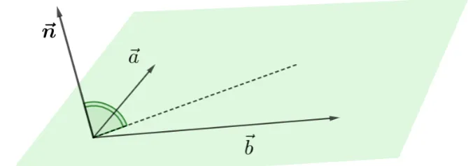
Geometric algebra has its origins in the work of Clifford and Grassman in the 19th century and is considered as a unified language for mathematics and physics. It is based on the notion of an invertible product of vectors that captures the geometric relationship between two vectors, i.e., their relative magnitudes and the angle between them [? ]. Some investigations have defined the properties of geometric algebra [? ?] applied to physics and engineering. Traditional concepts such as vector, spinor, complex numbers or quaternions are naturally explained as members of subspaces in geometric algebra. It can be easily extended in any number of dimensions, being this one of its main strengths. Because these are geometrical objects, they all have direction, sense and magnitude. The basics of GA properties are based on well established definitions around vectors. For example, a vector
a=α1e1+α2e2(a segment with direction and sense) can be multiplied by a vectorb=β1e1+β2e2in different ways, so the result has different meanings. In (2), the inner product is defined and the result is a scalar.
Figure 1.Outer product of vectorsaandb. The result is a vectorn, perpendicular to the plane formed byaandb
outerproduct (see figure1) is that the result is neither a scalar nor a vector, but a new quantity called bivector.
a∧b=kakkbksinϕe1e2 (3)
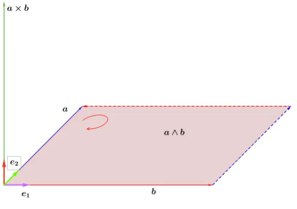
A bivector is known to have direction, sense and magnitude in the same way a vector has. It defines an area enclosed by the parallelogram formed by both vectors (see figure2). This product complies with the anti-commutative property, i.e. a∧b = −b∧a. A bivector is a key concept in geometrical algebra and cannot be found in linear algebra or vector calculus. The outer product of two vectors produces a new entity in a plane that can be operated like vectors, i.e., addition, product or even inverse. Like vectors, a bivector can be written as the linear combination of a base of bivectors.
Figure 2.Representation of a bivectora∧b
Finally, the third product between vectors is defined in (4) as thegeometric productand can be described as one of the major contributions in geometric algebra. Not only vectors can be multiplied geometrically, but bivectors and other entities, in general, can be used.
ab=a·b+a∧b (4)
The result is a linear combination of the inner product and the wedge product. Equation (4) can be expanded to further find out new insights.
A=ab=hAi0+hAi2= (α1β1+α2β2) + (α1β2−α2β1)e1e2 (5) wherehAi0is the scalar part andhAi2is the bivector part.
2.2. Application of geometric algebra to power systems
Recently, several researchs have proven that geometric algebra or Clifford algebra is a powerful and flexible tool for representing the flow of energy or power in electrical systems [? ? ]. Some authors have motivated the use of power theory based on geometric algebra as Physics’ unifying language, such that electrical magnitudes can be interpreted as Clifford multivectors [? ]. More specifically, Clifford algebra is a valid mathematical tool to address the multicomponent nature of power in non-sinusoidal contexts [? ? ?] and has been used for analysis of harmonics [?].
verification of the energy conservation law is only possible in sinusoidal situations [?]. To overcome these drawbacks, these authors proposed a new circuit analysis approach using geometric algebra to develop the most general proof of energy conservation in industrial building loads, with capability of calculating the voltage, current, and net apparent power in electrical systems in non-sinusoidal situations.
Different authors have proposed definitions to represent non-active power for distorted currents and voltages in electrical systems, although no single representation has been universally accepted. For example, in [?] a non-active power multivector from the most advanced multivectorial power theory based on the geometric algebra with the aim of analyzing the compensation of disturbing loads is presented, including the harmonic load compensation, identification, and metering between other applications. Other researches have shown that geometric algebra can be applied to analyze the apparent power defined in a poly-phase system having transmission lines with frequency-dependency under non-sinusoidal conditions [?].
2.2.1. Geometric apparent power
As several authors have shown, the use of apparent power loses its meaning under non-sinusoidal conditions, involving erroneous calculation of energy flows between the load and source. In contrast, [?] proposes the use of a new term called net apparent power or geometric apparent powerM. This concept is the result of the geometric product of voltage and current inGN domain (6).
M=ui=u·i+u∧i (6)
which result in a scalar and a bivector when the voltage and current are sinusoids
M=hMi0+hMi2 (7)
It can be easily shown from (7) and (1) that
P=hMi0 Q=khMi2k
(8)
sohMi0is the active power derived from the scalar part andkhMi2kis the reactive power derived from the bivector part of the net apparent power multivector.
For the non-sinusoidal case, i.e., when harmonics are present in the voltage and/or current, the apparent power loses its validity and onlyMcan reflect the exact flow of energy in the circuit. Consider a general voltage waveformu(t)
u(t) =
n
∑
i=1
ui(t) =α1cos(ωt) +β1sin(ωt) +
l
∑
h=2
αhcos(hωt) +
k
∑
h=2
βhsin(hωt) (9)
ϕc1(t) = √
2 cosωt ←→ e1
ϕs1(t) = √
2 sinωt ←→ −e2
ϕc2(t) = √
2 cos 2ωt ←→ e2e3
ϕs2(t) = √
2 sin 2ωt ←→ e1e3 ..
.
ϕcn(t) = √
2 cosnωt←→ n+1
VVV
i=2
ei
ϕsn(t) = √
2 sinnωt ←→ n+1
VVV
i=1
i6=2
ei
(10)
whereVVV
ei represents the product ofnvectors and the subscriptscandsdenote cosine and sine,
respectively. Using (10), any waveformx(t)can be translated to the geometric domainGN, so the final result for the voltage is
u=α1e1−β1e2+ l
∑
h=2
αh
h+1 ^
i=2
ei
+
k
∑
h=2
βh
h+1 ^
i=1,i6=2
ei
(11)
In (11), the transformation given in [?] has been used and is reproduced here to make this paper more readable. [?] also demonstrates that the admittance of typical passive load isYh =Gh+Bhe1e2, so the harmonic current associated toh-thvoltage harmonic is
ih = (Gh+Bhe1e2)uh (12)
and the total current
i=
n
∑
h=1
ih =ig+ib (13)
whereigis thein-phasecurrent whereibis the quadrature current. The geometric apparent power is then
M=ui=Mg+Mb=P+CNd+Mb (14)
where Mg is the in-phasegeometric apparent power, CNd is the degraded power (summation of cross-frequency products between voltage and current) andMbis the quadrature geometric apparent
power.
Based on equation (14) and (8) the power factor inGN domain can be defined as
p f = P
kMk =
hMi0
q
M†M
0
(15)
3. Problem description and solution strategy
This section describes the proposed problem in this research and details the characteristics of the genetic algorithm used to solve it.
3.1. Problem description
Power systems operating under harmonic distortion must be optimized to reduce power losses and improve power quality [? ? ]. Whether the system is linear or non-linear, it is necessary to provide reactances in parallel with the load in order to reduce these harmonics. The typical design of compensators is based on the knowledge of the susceptances of the system to different frequencies [?], something that is not easy to achieve when you have highly distorted systems. The main objective of non active power compensation is to minimize the source RMS current [?]. However, it is not a trivial task since it involves to determine which type of filter and characteristics of their components is more suitable for compensation purposes in a given circuit. For example, a capacitor with an optimal value connected in parallel to the load is an easy solution but this does not produce the absolute minimum of the distortion power [?], while other alternatives could improve it.
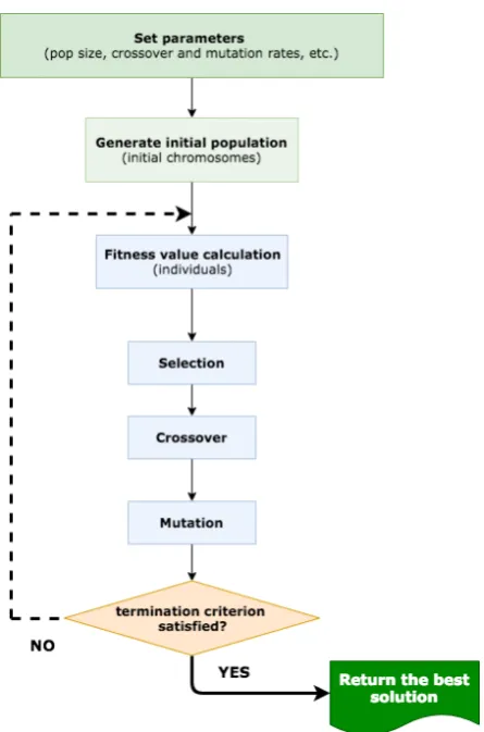
Figure 3.Flowchart of the genetic algorithm.
3.2. Solution approach
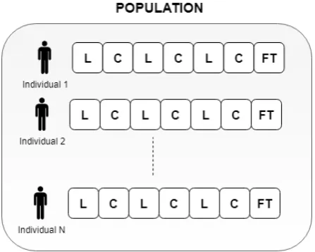
Genetic algorithms are optimization methods based on principles of natural selection and genetics [?]. Figure3shows the flowchart describing the operation of the genetic algorithm. It consists of a set (population) of solutions, each of which is called individual or phenotype, that evolve to reach solutions of high quality in terms of a fitness function. As an initialization step, genetic algorithm randomly generates a set of solutions to a problem (a population of genomes). As Figure4shows, each individual is represented by a string of real numbers. Specifically, the data structure of each individual consists of three possible values for inductorsL(Henry) and three possible values for capacitorsC (Farad). All or some of these values will be considered in the optimization process depending on the filter choosed, which will be specified in the FT field (filter type), as described below. The actual values that can be assigned to inductors and capacitors are preset between two limits (upper and lower), so that the search space of the evolutionary algorithm is limited within reasonable margins. After calculating the fitness values for all solutions in a current population, the individuals for mating pool are selected using the operator of reproduction according to a given fitness function defined for the problem to be solved. In our problem the fitness function is
min f(L,C) =Is(L,C) (16)
In this paper we have adapted a genetic algorithm solver for mixed-integer or continuous-variable optimization, constrained or unconstrained, included in the MATLAB Global Optimization Toolbox [? ]. This toolbox allows to solve smooth or non-smooth optimization problems with constraints using different mutation and crossover operators. The original source code has been adapted to deal with the problem at hand. It also has been adapted to take into account the particularities of the proposed problem through GA. More specifically, an opensource implementation of GA "Clifford multivector toolbox" has been used, available at https://sourceforge.net/projects/clifford-multivector-toolbox/. A preliminary sensitivity analysis has been performed to determine the parameters of the algorithm, such that the values used in our study are: Population size: 100 individuals; crossover rate: 0.8; mutation rate: 0.2; selection criteria: roulette wheel selection; termination criteria: 50 iterations.
Figure 4.Chromosome representation for the population. Note that the genes are real values for L, C and integer for FT (Filter Type).
4. Empirical study
This section presents the results obtained by the genetic algorithm in three different case studies.
4.1. Case studies
• Czarnecki’s case study [?]: This example consists of simple circuit with a harmonic polluted ideal voltage source of normalized frequencyω=1 rad/s
u(t) =100√2 cost+50√2 cos 2t+30√2 cos 3t (17) with an active powerP=344.23 W. Figure5(a) shows the circuit load, while Figure5(b) shows the solution found by Czarnecki withL1=5.906H,L2=19H,C1=0.034F andC2=0.012F, who compensate the reactive power of the harmonic components by the 1-port X of a precalculated admitance. The method proposed by Czarnecki was able to compensate the source RMS current to 3.10 A from the initial 12.24 A [?].
Using (10), the voltage inGN domain can be expressed as
1/12 F
6 H
1Ω
(a)Circuit proposed by Czarnecki
L1
C1
L2
C2
(b)Compensator layout
Figure 5.Load and compensator used by Czarnecki in [?].
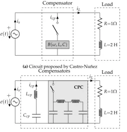
• Castro-Nuñez and Castro-Puche’s case study [?]: This example (already studied by Czarnecki) consists of a circuit with a highly distorted voltage source with fundamental plus 2 harmonics and a linear load, being the voltage
u(t) =100√2 sint+100
11 √
2 sin 11t+100
13 √
2 sin 13t (19)
which translates to
u=−100e2+100
11 12 ^
i=1,i6=2
ei+100
13 14 ^
i=1,i6=2
ei (20)
e(t)
is
iL icp
R=1Ω
L=2 H
+
B(ω,L,C)
Compensator Load
(a)Circuit proposed by Castro-Nuñez
CPC
e(t)
is
iL
Ccp
Lcp
icp
R=1Ω
L=2 H
+
Compensators Load
(b)Compensators proposed by Castro-Nuñez (LcpCcp) and Czarnecki (CPC)
Figure 6. Circuit with distorted voltage source and a linear load used by Castro-Nuñez and Castro-Puche [?].
• Castilla’s case study [?]: This example consists of a circuit with a distorted voltage source with three harmonics given by:
u(t) =200√2 cosωt+200
√
2 cos(3ωt−30) +100
√
2 cos(5ωt+30). (21)
which translates to
u=200e2+100 √
3e234+100e134+50 √
3e23456−50e13456 (22) with an uncompensated RMS current ofkIk = 4.21 A. Although the structure of this compensator was not described in the paper published by Castilla [?], this author indicated that it reduced the source RMS current to 3.21 A.
4.2. Filter optimization
The genetic algorithm has been adapted to manage different types of filters widely used in the literature for compensating purposes and mitigation of current harmonics. Based on equation (12), the admittance for a general loadYland harmonich, is equal to
Ylh =Glh+Blhe1e2=Glh+Blhe12 (23) If we connect a pure reactive impedance in parallel with the load for current compensation, its admittanceYcph will be
Ycph =Bcphe12 (24)
Zh =XLh+XCh =−hLωe12+ 1 hωCe12 Yh =
1
Zh =
1
−hLω+hω1C
e12
= hwC
h2ω2LC−1e12
(25)
So we need to make equalBcp=−Blfor every harmonichto fully compensate the quadrature term. For the opmital case, the total currentiis reduced toigsinceib+icpis equal to 0 after applying
Kirchhoff laws.
The following configurations were used based on very well-known type of filters:
• C-type filter: it is is mainly used for suppressing the low order of harmonics [?].
C
Figure 7.C-type filter.
• Series LC-type filter: this filter is also considered to reduce line current harmonics [?].
C L
Figure 8.Series LC-type filter.
• Parallel LC-type filter: it provides low impedance shunt branches to the load’s harmonic current, which allows to reduce the harmonic current flowing into the line [?].
C L
Figure 9.Parallel LC-type filter.
• Triple tuned filter: This type of filter is electrically equivalent to three parallel tuned filters connected in series [?].
L1
C1
L2
C2
L3
C3
• Foster’s filter: this filter combines in parallel single L-type and C-type filters and also parallel LC-type filters.
L1
C1 C2 L2 C3 L3
Figure 11.Foster’s filter.
• Czarnecki’s 4-elements filter: it is a filter that combines two L and two C elements using a series/parallel configuration [?].
C2
L2
C1
L1
Figure 12.Czarnecki’s 4-elements filter.
4.3. Simulation results
Tables1,2, and3show the results obtained by the genetic algorithm in the three case studies described above, being the RMS current through the supply source the objective to be minimized. The best, mean and standard deviation of 10 independent runs are provided.
Type of Filter
C Series LC Parallel LC Triple tune Foster Czarnecki 4
Best(A) 12.2409 7.5015 12.7235 3.0954 3.0948 3.0987
Mean(A) 12.2415 7.5017 12.7249 3.1040 3.1079 3.1454
Std. dev. 0.0008 0.0002 0.0011 0.0124 0.0155 0.0468
Table 1.Compensated RMS current (Iscp) obtained by the genetic algorithm in Czarnecki’s case study
[?].
C Series LC Parallel LC Triple tune Foster Czarnecki 4 Best(A) 38.0511 20.0275 75.5999 20.0288 20.0094 20.0271 Mean(A) 38.0513 20.0313 75.7476 20.5668 20.0807 20.0415
Std. dev. 0.0003 0.0030 0.1411 0.7039 0.0617 0.0150
Table 2. Compensated RMS current (Iscp) obtained by the genetic algorithm in Castro-Nuñez and
Castro-Puche’s case study [?].
Type of Filter
C Series LC Parallel LC Triple tune Foster Czarnecki 4
Best(A) 3.7938 3.5236 3.8242 3.2024 3.2131 3.5268
Mean(A) 3.7938 3.5437 3.8242 3.2613 3.2722 3.5313
Std. dev. 0.0000 0.0210 0.0000 0.0369 0.0304 0.0067
Table 3.Compensated RMS current (Iscp) obtained by the genetic algorithm in Castilla’s case study. [?
].
14
of
17
Table 4.Optimal values for L,C achieved by the genetic algorithm for the 3 cases of study and the 6 proposed filters.
Czarnecki Castro-Nuñez Castilla
C Series LC Parallel LC Triple Tune Foster Czarnecki 4 C Series LC Parallel LC Triple Tune Foster Czarnecki 4 C Series LC Parallel LC Triple Tune Foster Czarnecki 4
L1(H) - 10.2116 99.995 0.794 17.457 5.906 - 1.953 2.000 0.256 1.511 1.977 - 15.6537 10.000 0.082 10.000 9.998
L2(H) - - - 0.724 6.555 19.000 - - - 0.063 1.641 - - - - 0.072 6.651 9.903
L3(H) - - - 1.920 5.945 - - - - 0.020 1.198 0.320 - - - 0.021 0.660
-C1(µF) 0.010 43373.492 13.0128 264930.386 2991.689 34530.000 135667.470 224040.6422 304711.7123 650723.116 21800.000 172388.219 7.157 0.636 7.291 20.098 5.797 2.079
C2(µF) - - - 106280.564 59192.627 12880.000 - - - 985889.243 366000.000 50406.350 - - - 165.469 1.451 16.065
C3(µF) - - - 586142.767 26682.668 - - - - 89338.809 107600.000 - - - - 21.464 0.844
-Iopt(A) 12.240 7.501 12.723 3.095 3.094 3.098 38.051 20.027 75.599 20.028 20.009 20.027 3.793 3.523 3.824 3.202 3.213 3.526
doi:10.20944/preprints201902.0181.v1
Peer-reviewed version available at
Energies
2019
,
12
, 692;
values without compensation Is, the optimum current that a passive filtering can achieveIopt, that provided by each authorIauthand the optimum current obtained by applying the technique used in this workIGAcp. The value of the power factor for each of the above situations is also indicated plus the power factor without compensation using GA,PFGA. It should be noted that the power factor may differ between what is calculated by complex numbers and what is calculated by geometric algebra due to the different nature of the apparent powerSand the geometric apparent powerM. For the first case, the power factor is calculated asP/Swhile for the second case it isP/M. For example, for the Czarnecki case study, the apparent powerSwithout compensating is worth 1,417 VA while compensated is worth 358.8 VA. However, using geometric algebra the powerMis worth 1,842 VA and compensated is worth 359.25 VA. It should be noted that the final result of the compensation is quite similar since the proposed example is of low complexity as it only has 3 harmonics and low order. If we take into account the case of Castro-Nuñez or Castilla, the power of the proposed method is verified since with only 2 elements (LC filter series) or 3 elements, an almost optimal compensated current is obtained, unlike the original proposal of the author where the filter involved has many more elements and therefore, much less economic. It should also be noted that the methodology proposed by Castro-Núñez indicates the path to follow when it comes to compensate for the correct power terms,
Mb, which is not possible to cancel with the traditional power theory because it doesn’t account for
those terms arising from crossed products between voltage and currents.
Current Power factor
Is Iopt Iauth IGAcp PFs PFopt PFauth PFGA PFGAcp
Czarnecki 12.24 3.09 3.10 3.09 0.243 0.959 0.959 0.186 0.959 Castro-Nuñez 44.72 20.00 20.10 20.00 0.445 0.993 0.988 0.445 0.992 Castilla 4.21 3.20 3.21 3.20 0.630 0.829 0.829 0.630 0.829
Table 5.Comparison table for currents and power factor
5. Conclusions
In recent years, different authors have shown that geometric algebra, also known as Clifford algebra, can be applied to analyze electric circuits. Having in mind that different studies have shown that geometric algebra is more appropriate than the algebra of complex numbers for the analysis of circuits with non-sinusoidal sources and linear loads, this investigation is an important contribution in estimating the type of filter and its parameters to optimize the quadrature current in electrical circuits which leads to the compensation of new power terms like quadrature apparent powerMbnot included
in the commonly accepted definition of electrical power standards. The traditional compensation of reactive power is exceeded by the compensation of cross products between current and voltage that have not been previously taken into account. The proposed approach is based on the use of a genetic algorithm which is able to optimize the parameters of different types of passive filters. In particular, six widely-used filters (single-tuned, double-tuned, triple-tuned, damped-double tuned and C-type ones by regarding their contribution on the loading capability improvement of the transformers under non-sinusoidal conditions.
Appendix
A. General concepts
Given an ortho-normal base{σk}withk=1, ...,Nfor a vector spaceRN, it is possible to define a new space called geometrical algebraGN. This new space is characterized by bases not only composed of{σk}, but also of external products between these vectors. For example, in the case of a 3D Euclidean space, there is an ortho-normal base{σ1,σ2,σ3}whereσn2=1. Applying the concept of Grassmann
product or exterior product, you get
σl∧σm=σlσm=σlm (26)
which is a new entity, different from a scalar or a vector because
(σl∧σm)2= (σlσm)(σlσm) =σl(σmσl)σm=σl(−σlσm)σm=
=−(σlσl)2(σmσm)2=−(1)(1) =−1
(27)
σlσmsquares to−1 so we can conclude that we are facing a new element, which is called a bivector. In the same way, the external product of more than 3 vectors is called trivector, and in general, the product ofkvectors is calledk-vector. In this way, algebraG3can be developed with the base
{1,σ1,σ2,σ3,σ12,σ13,σ23,σ123} (28)
Generally speaking, the elements of a geometric algebra are called multivectors (M) and can be expressed as a linear combination of the different bases
M=hMi0+hMi1+hMi2+...+hMin = n
∑
k=0
hMik (29)
where eachhMik is an element of grade k, representing scalars (grade 0), vectors (grade 1), bivectors (grade 2) or in general,k-vectors (gradek).
B. Geometric operations
The geometric product is the cornerstone of geometric algebra and is indebted to the contributions of Grassman and Clifford. It is defined as the sum of the scalar product and the external product, and for the case of 2 vectorsviandvj
vivj=vi·vj+vi∧vj (30)
for the base vectorsσiandσjwithi6=j, we get bivectors
σiσj=σi·σj+σi∧σj=σi∧σj=σij (31)
base vectors anticommute fori6= jbecause
σiσj=σi∧σj=−σj∧σi=−σji (32)
On the other hand, unlike vectors which squares to 1, bivectors squares to -1
σijσij =σiσjσiσj=−σjσiσiσj=−σjσj=−1 (33)
M†=
∑
k=0
hM†ik = (−1)k(k−1)/2hMik (34)
The norm of a multivectorM(kMk) is always a scalar and can be obtained
kMk=
q
M†M
0=
q
MM†
0=
∑
khhMikhM†iki0 (35)
Author Contributions:Conceptualization, FGM and RB; Methodology, RB; Software, AA and FAC; Validation, AA, RB and FAC; Formal Analysis, FGM; Investigation, FGM and AA; Resources, FAC; Data Curation, RB; Writing—Original Draft Preparation, RB, FGM and FAC; Writing—Review & Editing, FGM, AA, FAC and RB; Visualization,FGM; Supervision, FGM; Project Administration, FGM and AA
Funding:This research received no external funding
![Figure 5. Load and compensator used by Czarnecki in [? ].](https://thumb-us.123doks.com/thumbv2/123dok_us/8055193.1342341/9.595.211.384.86.297/figure-load-and-compensator-used-by-czarnecki-in.webp)


![Table 2. Compensated RMS current (Iscp) obtained by the genetic algorithm in Castro-Nuñez andCastro-Puche’s case study [? ].](https://thumb-us.123doks.com/thumbv2/123dok_us/8055193.1342341/13.595.110.485.87.159/compensated-current-obtained-genetic-algorithm-castro-nunez-andcastro.webp)

