Article
Utility Perception in System Dynamics Models
§
Saeed P. Langarudi1,* and Isa Bar-On2
1 New Mexico State University; [email protected]
2 Worcester Polytechnic Institute; [email protected]
* Correspondence: [email protected]; Tel.: +1-508-471-4717
§ This paper is an extended version of our paper published in Langarudi, Saeed P., and Isa Bar-On. 2017. “Utility Perception in System Dynamics Models.” In Proceedings of the 35thInternational Conference of the System Dynamics Society, Cambridge, MA: System Dynamics Society..
Abstract:Utility perceived by individuals is believed to be different from the utility experienced by that individual. System dynamicists implicitly categorize this phenomenon as a form of bounded rationality and traditionally employ a simple smoothing function to capture it. We challenge this generalization by testing it against an alternative formulation of utility perception that is suggested by modern theories of behavioral economics. In particular, the traditional smoothing formulation is compared with the peak-end rule in a simple theoretical model as well as in a medium-size model of electronic health record implementation. Experimentation with the models reveals that the way utility perception is formulated is important and might affect behavior and policy implications of system dynamics models.
Keywords:utility; peak-end rule; smoothing; perception; system dynamics
1. Introduction
Decisions regarding preferences involve the utility derived from the preferred outcome. Utility in this context can be either experienced utility or decision utility, and there can be notable differences between the two [1–3].
Experienced utility is the pleasure (or its opposite) that we gain from an action at any moment. Decision utility is revealed by the choices we make, and is also called revealed preference. Experienced utility can be summarized over time to obtain the total utility as determined by some valid measure. For decision utility it has been shown that it is frequently disproportionally affected by the peak and end values of an experience, while duration of experience seems to be less significant [4,5].
System dynamics models represent utility-based decisions using the construct of perceived utility. Perceived utility (or perceived preference) is formulated as a first order smooth. One example is the reaction of customers to long delays in delivery. Customer satisfaction from delivery time (x) will be perceived ( ¯x) with a delay (T):
¯
xt+dt=xt¯ + xt−xt¯
T ·dt (1)
This perception of utility, is usually symmetrical and uniformly smoothed over a particular time period. As such, it is akin to the sum of experienced utilities. The representation of utilities used in system dynamics models (shown in Equation 1) is developed from the use of smooths in the formulation of perceived information. Perceived information includes an information delay (smooth) of the actual information to represent the discrepancy between actual information and what we represent as the information perceived by an agent at the moment of information reception. Such
formulation implies that duration of experience plays a key role in formation of perception. We can rewrite Equation1as follows:
¯
xt+dt= (1−α)xt¯ +αxt (2)
α= dt
T <0.25
Equation2implies that perceived utility (information) is a weighted average of two arguments. The first argument is the average perceived utility in the past – thus, taking duration of the experience into account. The second argument is the utility perceived from the last moment of the experience – which is called “end value” as we will see later. The weight of the arguments depends on our selection of averaging time (T). However,αcan never be greater than 25%1. This means that the smoothing
formulation always gives at least 75% (i.e. 1−α) of the weight to the average perceived utility in the
past which represents duration of the experience.
Decision utility is qualitatively different as it includes psychological factors. These may lead to a disregard of time duration and emphasis on extreme values and more recent experiences as formulated in the Peak-End rule. The Peak-End rule had originally been documented for pain experienced during medical procedures [6] where patients were asked during the procedure to rate the pain that they experienced during the procedure in fixed intervals. After the procedure the patients were asked to rate the total amount of pain that they had experienced during the procedure. The results indicated that this later measure was not reflective of the sum of the values during the procedure, but was better represented by the average of the peak and last values—thus the term Peak-End value. This Peak-End rule has since been documented for a range of situations [7–9]. Implementation of a peak-end formulation for preferences gives the following expression:
U= P+E
2 (3)
U - Perceived (remembered) utility
P - Utility from most intense experience (PEAK) E - Utility from most recent experience (END)
This formulation is substantially different from that of an averaged expression of utility (represented by Equation 2). Although both of these equations are weighted averages of two arguments one of which is “end value,” they differ in the second argument. For the smoothing formulation the second argument is average past utility, while it is peak - utility for the peak-end formulation. Furthermore, the weight of the arguments in the peak-end formulation (corresponding toαin Equation2) is always constant and equal to 50%. Thus, the peak-end formulation gives greater
weight to the end value than does the smoothing formulation in the averaging function. It also ignores duration of the experience and gives the remainder of the weight to only one instant of history which is when the peak utility happens.
In this paper we pose the question whether or not alternative formulations of utility functions for preference decisions will substantially alter the results of the modeling exercise and thus of the corresponding policy recommendations. We start with a simple theoretical model that focuses on a comparison between the traditional perceived utility (smooth) and the peak-end rule formulation.
1 Rule of thumb dictates that the simulation time step (dt) must be smaller than 25% of the smallest time constant in the
model in order to avoid integration errors and at the same time achieving a reasonable precision for the simulation. As a result, the ratio ofdt
This is presented in the following section. Next, the rule is applied to a medium size system dynamics model that has been already developed for addressing technological changes in healthcare settings [10]. The last section concludes the paper.
2. Peak-end value in a theoretical model
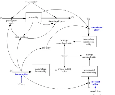
We first examine peak-end value formulation on a very simple example model. The model diagram is shown in Figure1. Equations of the model can be found in AppendixA. The model starts with an assumed “instant utility” that can be exposed to a test input. This is the exact utility individuals gain from an event. But what is perceived by them as “experienced utility” might be different. As mentioned in the Introduction, system dynamics models calculate this discrepancy between actual and perceived utility as simple smoothing. This is shown by “smoothed utility” in Figure1. As mentioned above, utility perception might be processed differently though. According to the peak-value hypothesis, utility that individuals perceive (“remembered utility”) is an arithmetic average of “peak utility” and “end utility.” Peak utility is the utility individuals gain from their most intense experience of an event. End utility, on the other hand, is the utility that individuals gain from their most recent experience of that particular event. In the model, we also calculate the average of each utility perception (“average smoothed utility” and “average remembered utility”) to better evaluate the effect of each on the overall state of the system.
peak utility picking new
peak discarding old peak
peak condition
<TIME STEP>
end utility
accumulated remembered
utility
remembered utility
accumulated instant utility instant utility
accumulated smoothed utility
smoothed utility average
remembered utility
average smoothed utility
average instant utility <Time>
<smoothing order> smooth time <Time>
Figure 1.Structure of a simple example of utility perception
2. It is assumed that instant utility changes between -1 and 1. Normal utility is equal to 0; minimum utility is equal to -1; and maximum is equal to +1.
1
.5
0
-.5
-1
1
3
5
7
9
11
13
15
17
19
Time (Week)
D
m
nl
instant utility : Current
smoothed utility : Current
remembered utility : Current
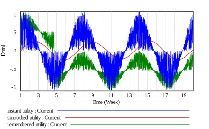
Figure 2.Behavior of the system in response to irregular oscillatory instant utility
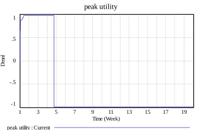
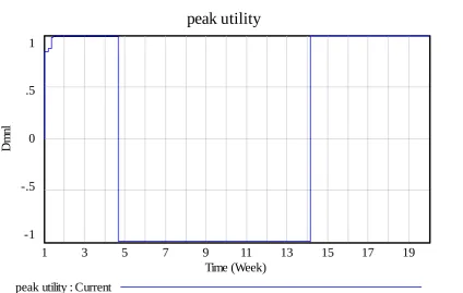
The numerical results show a systematic discrepancy between “smoothed utility” and “remembered utility.” Average smoothed utility for this case is 0.00661 whereas average remembered utility is -0.2869. The reason for such a significant discrepancy is that “peak” utility remains very low after week 5 as shown in Figure3. This, in fact, represents the worst experience of the individual (lowest utility) during the experiment.
If we repeat our experiment with a different random seed2we can observe a different behavior
as depicted in Figure4. On average, smoothed utility is 0.00359 and remembered utility is 0.00102 for this experiment. The discrepancy is not significant but the behavior is different.
In this case, the individual experiences a very intense experience around week 4 which remains in his (her) memory until week 14 when this extreme is replaced with a another intense experience which is positive this time. Changes in peak utility are depicted in Figure5.
An important implication of this experiment is that while the smoothed utility formulation always returns a more or less similar behavior, the remembered utility formulation may or may not be similar to instant and smoothed utility. Depending on instances of an individual’s experience during a particular event, remembered utility might differ dramatically from one instance to the other. In other words, qualitative dynamic behavior is not the only thing that matters; magnitude of difference between values of instances play a key role as well.
One may, nevertheless, argue that such variation in behavior of “remembered utility” might not be as decisive in a feedback-rich model where numerous negative feedback loops work to offset the irregularities. To address this argument the peak-end value formulation in comparison with the
2 Default random seed of the Vensim model is 1. To produce the alternative experiment, Vensim’s random seed of 123 is
peak utility
1
.5
0
-.5
-1
1
3
5
7
9
11
13
15
17
19
Time (Week)
D
m
nl
peak utility : Current
Figure 3.Change in peak utility in response to irregular oscillatory instant utility
1
.5
0
-.5
-1
1
3
5
7
9
11
13
15
17
19
Time (Week)
D
m
nl
instant utility : Current
smoothed utility : Current
remembered utility : Current
Figure 4.Behavior of the system in response to alternative irregular oscillatory instant utility
peak utility
1
.5
0
-.5
-1
1
3
5
7
9
11
13
15
17
19
Time (Week)
D
m
nl
peak utility : Current
Figure 5.Change in peak utility in response to alternative irregular oscillatory instant utility
3. Peak-end value in an EHR implementation model
In this section, peak-end value formulation of utility perception is applied to a system dynamics model that has already been developed to explain dynamics of electronic health records (EHR) implementation in healthcare settings [10].
The model includes many feedback loops representing complex interactions among different components of a healthcare organization. Figure 6 illustrates an aggregate overview of the EHR implementation model3. There are 9 interconnected modules in the model:
• Demandcalculates number of patients demanding healthcare services;
• Supplydetermines healthcare service capacity of the organization;
• Financeis an accounting module calculating costs, revenues, cash balance, and other financial measures;
• Quality of careaccounts for quality of healthcare services that the organization provides;
• Satisfactiontracks changes in satisfaction of patients and healthcare providers;
• Time allocation includes mechanisms by which physicians allocate their time between three major tasks: medical practice, learning and making use of the electronic health record system, and leisure;
• Data recordingtracks efforts made by physicians and nurses in capturing and recording digital medical data;
• Data incorporation represents level of activities of physicians and nurses in incorporating medical health records in actual medical practice;
• Experience shows skill and experience of physicians and nurses in working with the EHR system.
Figure 6.Sector view of the EHR implementation model [10]
One important goal of the model was to design policies in order to facilitate the EHR implementation processes. The original model is used to show that some specific settings are required to streamline the EHR implementation processes. Particularly, different payment systems were examined to identify effective settings:
• BASEis the payment system used in the default setting of the model. In this case, physicians are reimbursed based on a capitated payment system.
• FLEXPAYis a payment system similar to the BASE case but it also includes an additional bonus for physicians if their satisfaction declines.
• FIXPAYis a different payment system based on constant salary. In addition, physicians will receive extra bonus pay if their satisfaction declines.
• FIXPAY2is also based on constant salary but 20% higher than the FIXPAY case. Additional bonus will be paid to physicians if higher quality of care is observed.
There are 7 utility perception equations in the EHR implementation model:
• physician satisfaction from patient satisfaction,
• physician satisfaction from leisure,
• physician satisfaction from income,
• physician satisfaction from quality of care,
• patient satisfaction from quality of care,
• patient satisfaction from wait time, and
• patient satisfaction from visit time.
Each of these utilities then goes through the utility perception processes described in the previous section to yield perceived utility. A binary variable will be used to switch between traditional smoothing and peak-end value utility perception formulations.
Preliminary simulation results show significant discrepancy between outputs of the simple smoothing model and those of the peak-end model. One example of such results is illustrated in Figure7. While all four graphs show qualitatively different results for the peak-end value formulation than for the standard smoothing formulation, it is the financial balance that shows the implications most drastically. For the smoothing formulation Financial Balance shows increases with time, while the use of the Peak-End Value formulation shows a monotonic decrease in Financial Balance. But these results are derived from only one possible initial setup of the model and might not be a good reference for generalization. Indeed, we need a more comprehensive analysis in order to provide a meaningful argument.
Physician Time Spent on EHR 7 5.25 3.5 1.75 0 2 2 2 2
2 2 2 2 2 2 2 2 2 2 2
1 1
1
1
1 1 1
1 1 1 1 1 1 1 1
1 151 301 450 600
Time (Week) H ou r/ (W ee k* P eo pl e)
Simple Smoothing 1 1 1 Peak End Value 2 2 2 2
Patient Wait Time 5
3.75
2.5
1.25
0
2 2 2
2 2
2
2 2 2 2 2 2 2 2 2
1 1 1 1 1 1 1 1 1 1 1 1 1 1 1
1 151 301 450 600
Time (Week)
W
ee
k
Simple Smoothing 1 1 1 Peak End Value 2 2 2 2 Quality of Care
3
2.25
1.5
.75
0
2 2 2
2 2
2 2 2 2 2 2 2 2 2 2
1 1 1 1 1 1 1 1 1 1 1 1 1 1 1
1 151 301 450 600
Time (Week)
D
m
nl
Simple Smoothing 1 1 1 Peak End Value 2 2 2 2
Financial Balance 300 M 207.5 M 115 M 22.5 M -70 M 2 2 2 2 2 2 2 2 2 2 2 2 2 2 1
1 1 1 1 1 1
1 1 1 1 1 1 1
1 151 301 450 600
Time (Week)
$
Simple Smoothing 1 1 1 Peak End Value 2 2 2 2 Financial Balance 300 M 207.5 M 115 M 22.5 M -70 M 2 2 2 2 2
2 2 2
2 2 2
2 2 2 1
1 1 1 1 1
1 1 1 1 1 1 1 1
1 151 301 450 600
Time (Week)
$
Simple Smoothing 1 1 1 Peak End Value 2 2 2 2
Figure 7.Comparison between simulation outputs of the simple smoothing model and the peak-end model
We run 1000 Monte Carlo simulation with multivariate parameter settings. In these simulations, parameters of the model change in a wide range as shown in AppendixBso that the majority of parameter space is covered in the analysis. Each set of Monte Carlo simulations is repeated with a similar random seed on each model (simple smoothing and peak-end) for each payment scenario. Thus, at the end there will 8 (2 models multiplied by 4 payment scenarios) sets of Monte Carlo simulations (8000 runs, in total) to be used for comparative analysis.
While implementing the EHR system, performance measures must be also maintained. Overall performance of the EHR implementation system is assessed with four performance parameters, and they are:
• Average quality of care
• Average patient wait time
• Time spent on EHR
Comparing all data points for each pair of simulation runs would be a daunting task. So instead, we compare the results at the end of the simulation. In order to take dynamics of the results into account, average of the measures are used instead of their final value. This excludes “financial balance” which itself represents average of net profit over the simulation period. We compare the results in three different ways; i) looking for the number of results with significant differences, ii) looking for number of runs with improved performance in all 4 performance measures, and iii) number of runs with similar policy implications for both formulations.
3.1. Number of runs with significant difference in numerical results between the two formulations
The first perspective compares the numerical values of the four performance measures for each of the utility formulations. Here, we compare the simulation runs one by one and count those that have generated a significant difference between outputs of the simple smoothing model and those of the peak-end model.
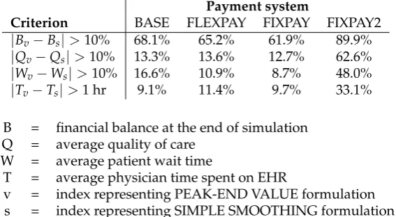
Table1summarizes the results. In the first row, we have the percentage of runs with a significant difference in financial balance generated by the simple smoothing model and by the peak-end model. For the base case, 68% of simulation runs generate a discrepancy greater than 10%. This figure changes to 65% if we switch to the FLEXPAY payment system and to 62% for the FIXPAY scenario. The figures go up to 90% for the FIXPAY2 payment system.
Table 1.Number of runs with significant difference in results between the two formulations
Payment system
Criterion BASE FLEXPAY FIXPAY FIXPAY2
|Bv−Bs|>10% 68.1% 65.2% 61.9% 89.9%
|Qv−Qs|>10% 13.3% 13.6% 12.7% 62.6%
|Wv−Ws|>10% 16.6% 10.9% 8.7% 48.0%
|Tv−Ts|>1 hr 9.1% 11.4% 9.7% 33.1%
B = financial balance at the end of simulation Q = average quality of care
W = average patient wait time
T = average physician time spent on EHR
v = index representing PEAK-END VALUE formulation s = index representing SIMPLE SMOOTHING formulation
The second row of the table shows the percentage of runs with a significant difference in average quality of care numbers generated by each utility formulation for the different payment systems. For the base case, FLEXPAY, and FIXPAY scenarios, about 13% of simulation runs yield a significant difference in average quality of care between the two utility perception models (simple smoothing and peak-end) i.e. greater than 10%. This figure is reaches about 63% for the FIXPAY2 system.
The third row of Table1reports the results for “average patient wait time.” The percentages of simulation runs that generate a difference greater than 10% in this performance measure between the two formulations are about 17%, 11%, 9%, and 33% for the base case, FLEXPAY, FIXPAY, and FIXPAY2, respectively.
In summary, the differences in performance measures for the two different utility formulations in the model are significant, especially for the case of FIXPAY2. This implies that for some particular initial settings of the models it will matter which utility perception formulation is employed. In other words, an alternative formulation of utility perception may lead to significantly different results.
3.2. Number of runs with improved performance in all 4 measures for each formulation
Now, we take a different look at the problem. This time, we count the number of simulation runs that have created any kind of improvement in all of the four performance measures for each of the different pay policies. More precisely, we first take the simple smoothing model; compare simulation outputs of the base case with one of the payment system, say FLEXPAY; and then, flag those runs that show improvement in all the performance measures. We then repeat the comparison between the base case and other payment systems (FIXPAY and FIXPAY2) and record the outcome. This same analysis is conducted on the peak-end model. Results are reported in Table2.
Table 2.Number of runs with improved performance in all 4 parameters for each formulation
Payment system Utility perception method FLEXPAY FIXPAY FIXPAY2 Simple Smoothing Model 28.9% 23.4% 41.3%
Peak-End Value Model 33.6% 31.9% 6.9%
For the simple smoothing model FLEXPAY shows improvement in all four parameters in about 29% of the runs; meaning that 29% of simulation runs show that this payment system can improve financial balance, quality of care, patient wait time, and EHR usage rate. FIXPAY has a lower improvement rate, about 23%. The FIXPAY2 system of payment, however, has a greater improvement rate of about 41%. A policy recommendation based on this model would be inclined towards FIXPAY2 rather than the other 2 policies.
On the other hand, with the peak-end model, the FLEXPAY payment system shows improvement about 34% of the times. FIXPAY shows improvement about 32% of the times . FIXPAY2 shows improvement in only 7% of the runs. Based on these results FIXPAY2 is definitely a rejected policy.
Thus while the smoothed utility formulation would recommend the FIXPAY2 policy the peak-end value formulation would likely reject this policy. These conflicting results imply that the selection of utility perception formulation may significantly impact policy recommendations of our models. One might reach dramatically different conclusions if the peak-end model is used over the simple smoothing model.
3.3. Number of runs with similar policy implications for both formulations
The results are reported in Table3. Similarity rates between the two models are strikingly low. For some policies such as FIXPAY2, there is a 32% chance of achieving similar outcomes from the simple smoothing and the peak-end models. When the FIXPAY policy is applied the two models yield more similar outcomes but even in this case only 57% of the simulation runs show similar policy implications.
Table 3.Number of runs with similar policy implications for both formulations
Payment system FLEXPAY FIXPAY FIXPAY2
Similarity rate 55.5% 57.1% 31.6%
4. Conclusion
In this paper we apply Kahneman’s decision utility to two system dynamics models and compare the results to those obtained from traditional perceived utility formulations. Specifically, we use the peak-end rule for comparison with the traditional smooth formulation. This rule, a result from behavioral economics, has been used successfully to describe preferences in a range of applications.
Experiments with a simple theoretical model that focuses on the different utility formulations indicate that there may be significant differences in model outcomes. The peak-end rule is then applied in a medium size model of electronic health record (EHR) implementation. The model has many (positive and negative) feedback loops and includes 7 utility perception equations and four different payment schemes One thousand Monte Carlo simulation runs are performed for each formulation and for each of the four payment policies, yielding 8000 total runs. Comparison between simulation runs across different models and different scenarios reveals that discrepancy in outputs of different models is considerable. The extent of discrepancy, however, depends on the initial setup of the models. Results also show that it is very likely that the two models lead to diametrically opposed policy recommendations.
Based on these results we conclude that different utility formulations for preferences actually matter. The point of this investigation was not to prove that the peak-end rule is necessarily the better formulation for the EHR model. Rather, we argue that the formulation of the decision utility for preferences may affect recommended policies. This situation is complicated as studies in behavioral economics seem to indicate that decision utility can, in addition, be influenced by time passed, repeated experiences and other psychological factors [11] for which there are no accepted utility formulations to date.
Despite the lack of consensus in utility formulation, we argue that the possibility of alternative formulations such as the peak-end rule (or others) should be investigated in cases where there is a reason to assume that they might be the dominant decision utility description or as a matter of good practice. These different formulations should be investigated together with a wide parameter space in order to identify potential policy recommendations that differ from those obtained with the traditional information. Much more work needs to be done to understand the effect of alternative utility formulations on the outcomes of system dynamics models, and a good starting point might be the investigation of generic structures and their sensitivity to such formulations.
Finally, we recommend that alternative formulations for utility perception be included in system dynamics software packages so that applications of theories such as peak-end value become readily available to modelers.
Acknowledgments:All sources of funding of the study should be disclosed. Please clearly indicate grants that you have received in support of your research work. Clearly state if you received funds for covering the costs to publish in open access.
Author Contributions:Saeed Langarudi and Isa Bar-On conceived and designed the experiments and wrote the paper; Saeed Langarudi performed the experiments and analyzed the data
Abbreviations
The following abbreviations are used in this manuscript:
MDPI: Multidisciplinary Digital Publishing Institute DOAJ: Directory of open access journals
TLA: Three letter acronym LD: linear dichroism
Appendix A. A: Equations of the peak-end module
accumulated instant utility = INTEG (instant utility,0)
Units: Dmnl
accumulated remembered utility = INTEG (remembered utility,0) Units: Dmnl
accumulated smoothed utility = INTEG (smoothed utility,0) Units: Dmnl
average instant utility = accumulated instant utility / Time Units: 1 / Week
average remembered utility = accumulated remembered utility / Time
Units: 1 / Week
average smoothed utility = accumulated smoothed utility / Time Units: 1 / Week
discarding old peak = peak utility * peak condition / TIME STEP Units: 1 / Week^2
end utility = instant utility Units: 1/ Week
instant utility = SIN(Time * max utility) * RANDOM UNIFORM(0, 1, random seed) Units: 1 / Week
max utility = 1
Units: 1 / Week
random seed = 1 Units: Dmnl
peak condition =
IF THEN ELSE(ABS(instant utility) >= ABS(peak utility), 1 , 0) Units: Dmnl
peak utility = INTEG (picking new peak-discarding old peak,0) Units: 1 / Week
Units: 1 / Week^2
remembered utility = (end utility + peak utility) / 2 Units: 1 / Week
smooth time = 2 Units: Week
smoothed utility =
SMOOTH N(instant utility, smooth time, 0, smoothing order) Units: 1 / Week
smoothing order = 1 Units: Dmnl
TIME STEP = 0.0078125
Units: Week
Appendix B. B: EHR Model’s Parameter Variation Range
PBPI=RANDOM_UNIFORM(0.00001,0.1)
PBPI --- Productivity booster per unit of investment (1 / $)
PCR=RANDOM_UNIFORM(0.1,0.9)
PCR --- Contact rate: indicates how frequently (potential and
/or current) patients meet each other (1 / Week)
PEHQ=RANDOM_UNIFORM(0,1)
PEHQ --- Elasticity of quality of care in response to physician satisfaction (Dmnl)
PEHRMC=RANDOM_UNIFORM(0.00001,0.01)
PEHRMC --- Unit cost of EHR maintenance ($ / (Week * Record))
PEIHS=RANDOM_UNIFORM(0,1)
PEIHS --- Elasticity of physician satisfaction in response to physician income (Dmnl)
PELHS=RANDOM_UNIFORM(0,1)
PELHS --- Elasticity of physician satisfaction in response to
physician leisure time (Dmnl)
PEQDI=RANDOM_UNIFORM(0,1)
PEQDI --- Elasticity of quality of care in response to effective usage of EHR (Dmnl)
PEQHS=RANDOM_UNIFORM(0,1)
PEQHS --- Elasticity of physician satisfaction in response to quality of care (Dmnl)
PEQPS --- Elasticity of patient satisfaction in response to quality of care (Dmnl)
PEQT=RANDOM_UNIFORM(0,1)
PEQT --- Elasticity of quality of care in response to average amount time a physician spends on a patient visit (Dmnl)
PESHS=RANDOM_UNIFORM(0,1)
PESHS --- Elasticity of physician satisfaction in response to patient satisfaction (Dmnl)
PETPS=RANDOM_UNIFORM(0,1)
PETPS --- Elasticity of patient satisfaction in response to time spent per patient (Dmnl)
PEWPS=RANDOM_UNIFORM(0,1)
PEWPS --- Elasticity of patient satisfaction in response to patient wait time (Dmnl)
PEXMC=RANDOM_UNIFORM(0,1)
PEXMC --- Exogenous management commitment to EHR implementation (Dmnl)
PFC=RANDOM_UNIFORM(10000,1000000) PFC --- Fixed costs ($ / Week)
PFINC=RANDOM_UNIFORM(5,20)
PFINC --- Normal financial coverage time (Week)
PMCPD=RANDOM_UNIFORM(0.0001,0.01)
PMCPD --- Supply cost of paper data records ($ / Record)
PMEXP=RANDOM_UNIFORM(100000,1600000)
PMEXP --- Initial (normal) marketing expenditure ($ / Week)
PMP=RANDOM_UNIFORM(1000,100000)
PMP --- Normal malpractice premium rate ($ / People)
PPB=RANDOM_UNIFORM(20000,400000)
PPB --- Maximum productivity booster investment per physician ($ / (People * Week))
PPHE=RANDOM_UNIFORM(100,1000)
PPHE --- Normal physian experience in using EHR (Hour / People)
PSCPV=RANDOM_UNIFORM(100,1000)
PSCPV --- Normal medical supply cost per patient visit ($ / People)
PTCPD --- Normal time a physician needs to capture and record a patient’s data (Hour /People)
PTIPD=RANDOM_UNIFORM(0.05,0.2)
PTIPD --- Normal time an average physician needs to incorporate a patient’s data into practice (Hour / People)
TAC=RANDOM_UNIFORM(6,24)
TAC --- Cost averaging time (Week)
TATSP=RANDOM_UNIFORM(2,8)
TATSP --- Time delay to adjust time spent per patient (Week)
TBD=RANDOM_UNIFORM(20,80)
TBD --- Productivity booster decay time (Week)
TEDI=RANDOM_UNIFORM(0.5,2)
TEDI --- Time delay for data incorporation to become effective (Week)
TEID=RANDOM_UNIFORM(5,20)
TEID --- Experience internalization delay (Week)
TENVP=RANDOM_UNIFORM(5,20)
TENVP --- Time delay to educate nurses for participating in patient visits (Week)
TEXMC=RANDOM_UNIFORM(10,200)
TEXMC --- Duration of exogenous management commitment to EHR implementation (Week)
TF=RANDOM_UNIFORM(2,20)
TF --- Time delay for financial state to affect expenditure (Week)
TFE=RANDOM_UNIFORM(50,200)
TFE --- Time constant to forget EHR experience and skills (Week)
TIMEP=RANDOM_UNIFORM(5,20)
TIMEP --- Perception time delay (Week)
TME=RANDOM_UNIFORM(10,40)
TME --- Time delay for marketing to become effective (Week)
TNV=RANDOM_UNIFORM(2,10)
TNV --- Time delay for nurses to be ready for help in patient visit (Week)
TPDL=RANDOM_UNIFORM(2000,4000)
TREP=RANDOM_UNIFORM(5,20)
TREP --- Time for reputation to evolve (Week)
TSS=RANDOM_UNIFORM(5,20)
TSS --- Time constant to smooth satisfaction (Week)
TTA=RANDOM_UNIFORM(2,8)
TTA --- Time delay to reallocate personal time (Week)
TWA=RANDOM_UNIFORM(5,20)
TWA --- Time delay to adjust wage rates (Week)
PPSW=RANDOM_UNIFORM(0,5)
PPSW --- Parameter affecting shape of the function FIPSW
[Paitient satisfaction from wait time] (Dmnl)
PPST=RANDOM_UNIFORM(0,5)
PPST --- Parameter affecting shape of the function FIPST
[Paitient satisfaction from visit time] (Dmnl)
PPSQ=RANDOM_UNIFORM(0,5)
PPSQ --- Parameter affecting shape of the function FIPSQ
[Patient satisfaction from quality of care] (Dmnl)
PHSQ=RANDOM_UNIFORM(0,5)
PHSQ --- Parameter affecting shape of the function FIHSQ [Physician satisfaction from quality of care] (Dmnl)
PHSL=RANDOM_UNIFORM(5,15)
PHSL --- Parameter affecting shape of the function FIHSL [Physician satisfaction from leisure] (Dmnl)
PHSI=RANDOM_UNIFORM(0,5)
PHSI --- Parameter affecting shape of the function FIHSI [Physician satisfaction from income] (Dmnl)
PHSP=RANDOM_UNIFORM(0,5)
PHSP --- Parameter affecting shape of the function FIHSP [Physician satisfaction from patient satisfaction] (Dmnl)
TPR=RANDOM_UNIFORM(30,100)
TPR --- Time delay for patients to return to the system (Week)
PEPB=RANDOM_UNIFORM(0.01,0.5)
PEPB --- Productivity elasticity of productivity booster (Dmnl)
TPHA=RANDOM_UNIFORM(5,20)
TSDS=RANDOM_UNIFORM(1,4)
TSDS --- Time to smooth desired number of staff (Week)
References
1. Kahneman, D.; Wakker, P.P.; Sarin, R. Back to Bentham? Explorations of Experienced Utility.The Quarterly Journal of Economics1997,112, 375–405. bibtex: kahneman_back_1997.
2. Kahneman, D. Experienced utility and objective happiness: A moment-based approach. The psychology of economic decisions2003,1, 187–208. bibtex: kahneman_experienced_2003.
3. Kahneman, D.; Thaler, R.H. Anomalies: Utility Maximization and Experienced Utility.Journal of Economic Perspectives2006,20, 221–234. bibtex: kahneman_anomalies:_2006.
4. Fredrickson, B.L.; Kahneman, D. Duration neglect in retrospective evaluations of affective episodes. Journal of Personality and Social Psychology1993,65, 45. bibtex: fredrickson_duration_1993.
5. Kahneman, D.; Fredrickson, B.L.; Schreiber, C.A.; Redelmeier, D.A. When More Pain Is Preferred to Less: Adding a Better End.Psychological Science1993,4, 401–405.
6. Redelmeier, D.A.; Kahneman, D. Patients’ memories of painful medical treatments: real-time and retrospective evaluations of two minimally invasive procedures. Pain1996,66, 3–8.
7. Stone, A.A.; Broderick, J.E.; Kaell, A.T.; DelesPaul, P.A.E.G.; Porter, L.E. Does the peak-end phenomenon observed in laboratory pain studies apply to real-world pain in rheumatoid arthritics? The Journal of Pain 2000,1, 212–217.
8. Clark, A.E.; Georgellis, Y. Kahneman meets the quitters: peak-end behaviour in the labour market; CNRS and DELTA, working paper, 2004.
9. Langer, T.; Sarin, R.; Weber, M. The retrospective evaluation of payment sequences: duration neglect and peak-and-end effects. Journal of Economic Behavior & Organization2005,58, 157–175.
10. Langarudi, S.P.; Strong, D.M.; Saeed, K.; Johnson, S.A.; Tulu, B.; Trudel, J.; Volkoff, O.; Pelletier, L.R.; Lawrence, G.; Bar-On, I. Dynamics of EHR Implementations. The 32nd International Conference of the System Dynamics Society; System Dynamics Society: Delft, Netherlands, 2014. bibtex: langarudi_dynamics_2014.
![Figure 6. Sector view of the EHR implementation model [10]](https://thumb-us.123doks.com/thumbv2/123dok_us/8062804.1343952/7.595.84.516.87.395/figure-sector-view-ehr-implementation-model.webp)