Advances in Graph-Cut Optimization: Multi-Surface Models, Label Costs, and Hierarchical Costs

(1)

Western University Western University

Scholarship@Western

Electronic Thesis and Dissertation Repository

9-15-2011 12:00 AM

Advances in Graph-Cut Optimization: Multi-Surface Models, Label

Costs, and Hierarchical Costs

Andrew T. Delong

University of Western Ontario

Supervisor Yuri Boykov

The University of Western Ontario Graduate Program in Computer Science

A thesis submitted in partial fulfillment of the requirements for the degree in Doctor of Philosophy

Follow this and additional works at: https://ir.lib.uwo.ca/etd

Part of the Artificial Intelligence and Robotics Commons, Discrete Mathematics and Combinatorics Commons, Other Statistics and Probability Commons, and the Theory and Algorithms Commons

Recommended Citation Recommended Citation

Delong, Andrew T., "Advances in Graph-Cut Optimization: Multi-Surface Models, Label Costs, and Hierarchical Costs" (2011). Electronic Thesis and Dissertation Repository. 298.

https://ir.lib.uwo.ca/etd/298

This Dissertation/Thesis is brought to you for free and open access by Scholarship@Western. It has been accepted for inclusion in Electronic Thesis and Dissertation Repository by an authorized administrator of

(2)

ADVANCES IN GRAPH-CUT OPTIMIZATION: MULTI-SURFACE

MODELS, LABEL COSTS, AND HIERARCHICAL COSTS

(Spine title: Advances in Graph-Cut Optimization)

(Thesis format: Monograph)

by

Andrew Delong

Graduate Program in Computer Science

A thesis submitted in partial fulfillment

of the requirements for the degree of

Doctor of Philosophy

The School of Graduate and Postdoctoral Studies

The University of Western Ontario

London, Ontario, Canada

(3)

THE UNIVERSITY OF WESTERN ONTARIO

School of Graduate and Postdoctoral Studies

CERTIFICATE OF EXAMINATION

Supervisor:

. . . . Dr. Yuri Boykov

Examiners:

. . . . Dr. Roberto Solis-Oba

. . . . Dr. Éric Schost

. . . . Dr. Hristo S. Sendov

. . . . Dr. Brendan J. Frey

The thesis by

Andrew Thomas Delong

entitled:

Advances in Graph-Cut Optimization: Multi-Surface Models, Label Costs, and Hierarchical Costs

is accepted in partial fulfillment of the requirements for the degree of

Doctor of Philosophy

. . . . Date

. . . . Chair of Thesis Examination Board

(4)

Abstract

Computer vision is full of problems that are elegantly expressed in terms of mathematical optimization, orenergy minimization. This is particularly true of “low-level” inference prob-lems such as cleaning up noisy signals, clustering and classifying data, or estimating 3D points from images. Energies let us state each problem as a clear, precise objective function. Min-imizing the correct energy would, hypothetically, yield a good solution to the corresponding problem. Unfortunately, even for low-level problems we are confronted by energies that are computationally hard—often NP-hard—to minimize. As a consequence, a rather large portion of computer vision research is dedicated to proposing better energies and betteralgorithmsfor energies. This dissertation presents work along the same line, specifically new energies and algorithms based ongraph cuts.

We present three distinct contributions. First we consider biomedical segmentation where the object of interest comprises multiple distinct regions of uncertain shape (e.g. blood vessels, airways, bone tissue). We show that this common yet difficult scenario can be modeled as an energy over multiple interacting surfaces, and can be globally optimized by a single graph cut. Second, we introduce multi-label energies withlabel costsand provide algorithms to minimize them. We show how label costs are useful for clustering and robust estimation problems in vision. Third, we characterize a class of energies withhierarchical costsand propose a novel

hierarchical fusionalgorithm with improved approximation guarantees. Hierarchical costs are natural for modeling an array of difficult problems,e.g. segmentation with hierarchical context, simultaneous estimation of motions and homographies, or detecting hierarchies of patterns.

Keywords: Energy minimization, graph cuts, discrete optimization, metric labeling, min-imum description length, segmentation, biomedical imaging, robust estimation, multi-view reconstruction.

(5)

Co-Authorship Statement

Chapters 1 and 2are my own original work in summarizing the relevant background.

Chapter 3 was a collaborative effort with my advisor, Yuri Boykov. He recognized that the high-level ideas of Liet al.[102] could be applied in a more straight-forward manner. We then developed the technical ideas together. I went on to create the examples, the code, some extensions, and ultimately wrote the bulk of our paper [36].

Chapter 4is about “label costs” and was a close collaboration with Anton Osokin, Hossam Isack, and Yuri Boykov. The homography detection and motion estimation applications were based on earlier work by Hossam Isack and Yuri Boykov on energy-based methods for multi-model fitting [68, 70]. I proposed the main technical idea that allows “label costs” and “label subset costs” to be optimized by theα-expansion algorithm. I then researched the related work on facility location and relevant high-order potentials; I am primary author of all related text. I programmed the C++/MATLAB library on which our work was based, starting from Olga Vek-sler’s publicα-expansion code. I collaborated with Anton Osokin on the approximation bound, and I designed the worst-case examples. Hossam Isack performed all the motion estimation and homography detection experiments specifically for this project; he and Yuri Boykov are primary authors of Section 4.7. Anton Osokin and Yuri Boykov are the primary authors of Sections 4.5.1 and 4.6.2—I merely helped to refine the presentation.

Chapter 5 is about energies with “hierarchical costs” and was developed for a pattern recognition project with Lena Gorelick, Olga Veksler, and Yuri Boykov. I proposed the hierar-chical fusionalgorithm, gave a formal characterizations of “hierarchical costs,” and developed all the proofs as they appear here. Theorem 5.15 uses ideas from a proof that Olga Veksler developed for a special case. I worked with Lena Gorelick on a prototype implementation of hierarchical fusion. Though we performed some experiments using this approach, they are part of a very complex application-oriented work [59] that is not part of this dissertation.

(6)

Dedication

To my loving parents,

who took a chance all those years ago.

And in memory of Kyle.

(7)

Acknowledgements

I owe so much to my advisor, Yuri Boykov, and to my informal co-advisor, Olga Veksler. Yuri has had an extraordinary (extraordinarious!) influence on my interests, my work ethic, my sense of humour, and my opportunities in life. I’m lucky to have an advisor who works out of genuine curiosity and a passion for research, and who knows how to have a measure of fun in doing it. It is hard to find words to thank Olga for all the ways she has helped me, both remembered and forgotten. I will never forget the time and genuine care that Yuri and Olga invested in me as mentors, and as friends. I think, through them, I gained a better sense for what is important, and what is not. Wherever I go next it will not be the same. _Spasibo.

I want to thank the many friends I made in the UWO vision group these last few years. I remember how surprised and happy I was to find out that Lena Gorelick was joining our group. Working with her has been great for me—lots of cool ideas bouncing around—and having fun with Lena and her husband Shachar has been even better. The last couple of years I’ve also enjoyed talking to Frank Schmidt each day, and learning how to express my complex feelings for Sarah Palin: a mix of pity, attraction, and Schadenfreude (Shaden = damage, Freude = joy). I particularly miss the time when Victor Lempitsky was visiting our group, and I am very lucky to have the hospitality and friendship that he and his wife (Victor’s-Olga) have shown me. I likewise miss the time that Olivier Juan was here, and wish he and his wife Charlotte the best in their new life as parents. Other fun and interesting visitors I’ve gotten to know include Carl Olsson and Anton Osokin. It was also a great pleasure to know June (have fun at Google!) and Hossam (have fun with Yuri!). Good luck to the Iranian club, Paria, Taha and Vida. Thanks also Mark Brophy for rare indulgences into politics and philosophy.

I also enjoyed the warm hospitality of Daniel Cremers, his wife Lena, and their adorable daughter while I stayed in Germany—thank you. I’d like to thank Jing Yuan and his family for their hospitality as well.

When first I arrived in London it was not the best of times for me, until I met great friends like Mike & Jasna, Santoni-san, Dan Siemon, Micah, Gaston & Alex, Franzi & Carsten, Ryan looks-hot-as-a-woman Demopoulos, Beth, Nathan, Angela, Shayne, Freddie and many others along the way. We had lots of fun, especially in 240, and it’s been bitter sweet to see everyone graduate and move on or get buried under their work.

I appreciate the advice and hard work of my thesis committee, professors Brendan Frey, Hristo Sendov, Éric Schost, and especially Roberto Solis-Oba who was meticulous and served on both my PhD and MSc committees. Also thanks to Cheryl for helping me out all those years and to Janice for laughing at my self-conscious jokes.

Last I want to thank my parents for being honest, hard-working, curious people. They make having integrity seem effortless. I’ve never figured out how they do that.

Graduate school has been a wonderful time, and a difficult time, in my life—but I would not trade these years for anything. I have been so fortunate, to have know all these persons, and to have had such freedom. I’ll try to hold on to that thought for a while.

(8)

List of Figures

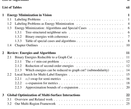
1.1 Example labeling problems: model fitting, semi-supervised learning, and

im-age/mesh segmentation. . . 2

1.2 Illustration of coherent (or ‘smooth’) labelings. . . 3

1.3 Semi-supervised learning as a labeling problem with coherence. . . 4

1.4 Dynamic programming example on a chain and on a tree. . . 7

2.1 Examples-tmin cut problem instance. . . 12

2.2 Examples of possibleαβ-swap moves. . . 17

2.3 Examples of possibleα-expansion moves. . . 19

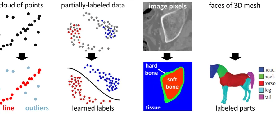
3.1 Bone segmentation from MRI data: a motivating example for multi-surface segmentation. . . 23

3.2 Illustration of the multi-surface segmentation method of Liet al. . . . 24

3.3 How method of Liet al.can be reduced to a single graph cut. . . 25

3.4 Standard binary segmentation model versus our multi-region model. . . 26

3.5 Graph construction for ‘containment’ interaction. . . 27

3.6 User-assisted segmentation of knee joint. . . 31

3.7 User-assisted cardiac segmentation. . . 31

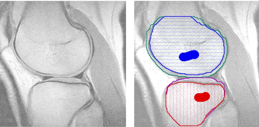
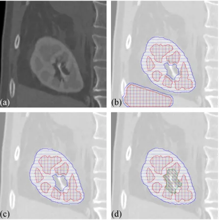
3.8 Automatic kidney segmentation. . . 32

3.9 Example of thescene layout estimationapplication. . . 33

3.10 Interaction graph for scene layout. . . 33

3.11 Experimental results for scene layout. . . 35

3.12 Illustration of how interaction causes local minima for αβ-swap, and makes α-expansion inapplicable. . . 36

3.13 Applying ‘QPBO’ to handle non-submodular interactions. . . 37

4.1 Motion segmentation with smooth costs and label costs. . . 40

4.2 Homography detection with smooth costs and label costs. . . 40

4.3 Unsupervised segmentation with smooth costs and label costs. . . 41

4.4 Directed graph construction to encode label cost insideα-expansion step. . . . 45

4.5 Undirected graph construction to encode label cost insideα-expansion step. . . 45

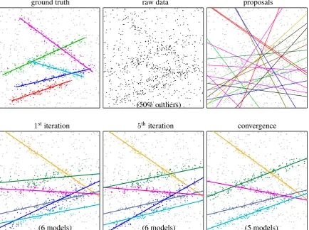
4.6 Illustration ofPEARLwith label costs on 2D multi-line fitting. . . 55

4.7 Energy-vs-time plot showing progress ofPEARLalgorithm on line fitting. . . 57

4.8 Energy-vs-time plot showing progress ofPEARLalgorithm on image segmen-tation. . . 58

(11)

4.9 Behaviour ofK-means versusweightedK-means. . . 62

4.10 Table of synthetic Gaussian mixture-model results comparing standard EM al-gorithm, standardK-means algorithm,PEARL, and EM with Dirchlet prior. . . . 64

4.11 Hard cases forK-means and for the EM algorithm. . . 66

4.12 Similarities between PEARLwith label costs and EM with Dirichlet prior. . . 67

4.13 Demonstration of lineinterval-fitting via PEARLwith label costs. . . 70

4.14 Circle-fitting using PEARLwith label costs. . . 70

4.15 Unsupervised image segmentation results. . . 72

4.16 Illustration of how low energies correspond to good homography detection re-sults. . . 75

4.17 Comparison of discrete algorithm variants on homography detection. . . 76

4.18 Comparison of discrete algorithms on rigid motion estimation. . . 78

5.1 The structure of anh-metric smooth cost matrix. . . 85

5.2 The structure of anh-Potts smooth cost matrix. . . 86

5.3 Example of fusing two labelings. . . 88

5.4 Depiction of hierarchical fusion algorithm on a tree. . . 89

5.5 Example ofh-fusion bound coefficientcfor various trees andh-metrics. . . 92

5.6 Conceptual depiction of hierarchical label costs for multi-class model fitting. . . 97

5.7 Conceptual depiction of label costs for fitting hierarchies of geometric models. . 107

(12)

List of Algorithms

1 The general LOCALSEARCHprocedure . . . 15

2 Theαβ-SWAPalgorithm. . . 18

3 Theα-EXPANSIONalgorithm. . . 19

4 The GREEDYUFL algorithm foruncapacitated facility location. . . 52

5 ThePEARLalgorithm for robust multi-model estimation. . . 54

6 Theh-FUSIONalgorithm (recursive) . . . 90

7 The SETUPFUSIONprocedure without label costs . . . 90

8 The SETUPFUSIONprocedure with label costs . . . 100

(13)

List of Tables

1.1 Special cases of the MAP-MRF energy, with exact/approximate algorithms for each case, and lists of typical applications. . . 9

(14)

Chapter 1 Energy Minimization in Vision

Broadly speaking, this dissertation is aboutenergy minimizationin computer vision. In com-puter vision anenergyis simply a mathematical objective function that we wish to extremize. For example, the energyE(x) = (x−5)2 _{+ (}_x₋₃₎2 _{has a minimum value of}₂ _at_x∗ _{= 4}_.

The specific use of the word ‘energy’ suggests an objective function that has its origins in sta-tistical physics—typically an unconstrained objective function where variables ‘interact’—but this connotation is not essential to our work. Rather, the important thing to understand is that a huge number of problems in vision areinference problems where the most likely explana-tion for the data can be found by minimizing a corresponding energy. For example, if we assume5and3are samples from a normal distribution, then thex∗ that minimizesE(x)is a maximum-likelihood estimate of the distribution’smeanparameter.

Of course, the inference problems in vision tend to be very complex and involve hundreds or even millions of inter-dependent variables. Some energies precisely model the desired in-ference problem, while others are merely a coarse approximation. Some energies are easy to optimize (e.g. convex functions) while others are known to be NP-hard. Once an accurate energy and a satisfying algorithm are both available, the associated inference problem is es-sentially solved. Researchers can then either improve the model or move on to other, more difficult problems.

Many of the most important developments in computer vision began with a proposal for a better energy, a better algorithm for an energy, or a combination of both. Good examples are [110, 132, 24, 83]. This dissertation is a small contribution in the same vein: we describe new energies that have useful interpretations, along with algorithms that are both effective in theory and fast in practice. We specifically focus on discrete labeling problems of the kind described in the following section.

1.1 Labeling Problems

A labeling problem is, roughly speaking, the task of assigning an explanatory ‘label’ to each element in a set of observations. Many classical clustering problems are also labeling problems because each data point is assigned a cluster label. To describe a labeling problem one needs a set of observations (the data) and a set of possible explanations (the labels). A discrete

(15)

2 CHAPTER1. ENERGY MINIMIZATION INVISION

cloud of points

tissue soft bone hard bone

line outliers

faces of 3D mesh image pixels

partially-labeled data

learned labels labeled parts

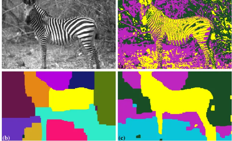
Figure 1.1: Example labeling problems. Given some input data, the goal is to assign an explanatory label to each input element. For example, if the data are 2D points then we may wish to classify them according to geometric models (points belonging to the same line). If the data comes partially-labeled, we can infer the remaining labels as in semi-supervised learning. (yinyang from [42], horse from [76].)

labeling problem associates one discrete variable with each datum, and the goal is to find the best overall assignment to these variables (a ‘labeling’) according to some criteria. In computer vision, the observations can be things like pixels in an image, salient points within an image, depth measurements from a range-scanner, or intensity measurements from CT/MRI. The labels are typically either semantic (car, pedestrian, street) or related to scene geometry (depth, orientation, shape, texture). Figure 1.1 depicts a few such possibilities.

We use the following notation for labeling problems throughout the dissertation. The set

P indexes the observations, and the label set Lindexes the explanations. The set of discrete variables is {fp}p_∈P where each fp is allowed to take one value from the set L. A discrete

labelingis the complete mapf :P → Lthat assigns to each elementp ∈ P a corresponding labelfp. For example, ifP = {p, q}andL = {ℓ1, ℓ2, ℓ3}, then labelingf = (ℓ3, ℓ1)says that fp =ℓ3andfq =ℓ1. If we instead letP index the pixels of a100×100image and there are two

labelsL ={object, background}, then this is a standard “binary segmentation” scenario with

210,000 _{possible labelings. In general we have}_|L||P| _{possible labelings (configurations of} _f_),

and we prefer one labeling over another based on some application-specific criteria.

Data-driven criteria In computer vision we try to make sense of the input data. This means that every labeling problem must be formulated so that the data influences the outcome. For example, if our100×100image is an X-ray and a particular pixelp∈ P is brightly coloured, then our labeling problem should prefer a labeling withfp =boneover one withfp =tissue.

If the image were of an outdoor scene instead, then we would expect blue pixels to prefer labels likeskyorwaterand green pixels to prefer labels likegrassorleaves. This is the most rudimentary kind of data-driven criterion possible, where each discrete variablefp derives its

(16)

1.1. LABELING PROBLEMS 3

image bad labeling “smooth” good labeling

“noisy”

Figure 1.2: Suppose we want to isolate a bright object on a dark background. The simplest approach is to choose a labeling based on data-driven pixel preferences,i.e.bright pixels choose object, dark pixels choose background. However, the resulting contour will often be complex and noisy (left). When we knowa priorithat the object’s shape should have a smooth, ’blobby’ contour (cars, people, buildings) then we should prefer a labeling that satisfies this assumption (right). Each pixel in a smooth labeling is highly correlated with its nearest neighbours in the spatial grid,e.g.the magnified regions contain 15 transitions versus only 5 transitions.

Regularization criteria Some labelings are more likely to be correct a priori. When we explicitly prefer some kinds of labelings over others, irrespective of the data, these criteria are called regularizers. The most prominent example in computer vision is a preference for

spatially coherent labelings. The idea is that, for most computer vision problems, coherent (“smooth”) labelings are much more likely to be a correct explanation of the data than are incoherent (“noisy”) labelings. For example, consider the binary image labelings below.

smooth / coherent semi-coherent incoherent / noisy

(car? bed? heart?) (tree? rivers? arteries?) (random noise? snow?)

We know from experience that objects in photographs and in medical data correspond to coher-ent labelings more often than not; the truth of this claim varies from application to application, but in computer vision it has become a rule of thumb. It holds true because data in computer vision tends to be highly correlated in space. For example ifp, q ∈ P are adjacent pixels in an X-ray image then one can expectfp =bone⇔ fq =bonewith high probability, regardless of

the data. The same cannot be said ifpandqare very far apart in the image, because such pixels are not directly correlated in practice. It turns out that sucha prioriassumptions, orpriors, are very important—often crucial—in many vision applications [54, 103].

(17)

partially-labeled data computed neighbours N optimal clustering

Figure 1.3: Given a set of points, some of which are labeled,semi-supervised learningasks us to choose the most probable label for each unlabeled point. Above we see 4 pre-labeled points (2white, 2black). To cluster the points, Blum & Chawla [17] compute a neighbour graph (e.g. nearest-neighbour, De-launay triangulation) and then find a labeling that is smooth with respect to that connectivity. In other words, constrained clustering problems can be solved using the same criterion as for image segmenta-tion [42].

close-up of the pixel grid also suggests a way to make the notion of smoothness more precise: smoothness implies fewer label transitions between neighbouring variables. This characteri-zation of smoothness is standard in computer vision and we formalize it in the next section. Figure 1.3 explains how this same smoothness criterion can be used in semi-supervised learn-ing [17, 140, 167]—an important labellearn-ing problem that, on the surface, seems entirely different from segmentation [42].

1.2 Labeling Problems as Energy Minimization

We now express some standard data-driven and regularization criteria as concrete energy terms. An energy term is an expression, dependent on labeling f, that is added linearly in the energy. Breaking an energy into terms means expressing it in the form

E(f) = term1(f) + term2(f) +. . .

Each energy term basically votes on how much it likes labelingfor some subset of its variables. If a particular term evaluates to a small numerical value, then this meansf reasonably satisfies the corresponding criterion. MinimizingE(f)thus finds a compromise among all the labeling criteria in the energy.

For example, suppose we have P = {p, q, r}and two possible labelsL = {ℓ1, ℓ2}. If we

sayDp(ℓ)is the cost of assigningfp =ℓ based on the data, then we insert expressionDp(fp)

as a term in the energy. Assume our energy contains only the data terms shown below, where the table gives individual assignment costs based on the data.

E(f) =Dp(fp) +Dq(fq) +Dr(fr)

0 6 0

10 5 5

data costs

ℓ₁ ℓ₂

p q r

(18)

1.2. LABELING PROBLEMS ASENERGYMINIMIZATION 5

can be minimized independently. (Minimizing such an energy is equivalent to “thresholding” techniques from the early days of image processing.)

Now suppose we wish to incorporate the prior knowledge that some of the observations are directly correlated with each other; specifically we wantpcorrelated with q andq correlated withr. We can incorporate this ‘coupling’ of variables by adding energy terms that explicitly encouragefp =fq andfq=fr. We refer to these assmooth termsand denote them byV.

E(f) =Dp(fp) +Dq(fq) +Dr(fr) +V(fp, fq) +V(fq, fr)

In the simplest case we use the delta functionV(ℓ, ℓ′) =δ(ℓ ̸=ℓ′)whereδis1if its condition is true, and 0 otherwise. The old optimum of f = (ℓ1, ℓ2, ℓ1) now evaluates to E(f) = 7,

whereas the new optimumf∗ = (ℓ1, ℓ1, ℓ1)evaluates toE(f∗) = 6. The smooth terms

encour-aged the labeling to becoherent(consistent) so that fluctuations caused by noisy data costs are smoothed out. Note that the the optimal label assignments can no longer be solved indepen-dently, and must somehow be minimized jointly. It is not entirely obvious how to minimize such energies in general. For problems with thousands of inter-dependent variables we will need fast, specialized algorithms to computef∗, or at least an approximation thereof.

LetN denote the pairs of observations we knowa priorito be correlated, for example in our 3-variable problem we used N = {{p, q},{q, r}}. We refer to N as the neighbour set

throughout. Common neighbour sets in vision are depicted as graph edges below.

4-connected grid 8-connected grid non-uniform, distance-based

Further assume that each unordered pair pq ∈ N interacts using its own smooth term where, for example,Vpq might be a different strength thanVqr. We can write this class of energies as

E(f) = ∑ p∈P

Dp(fp) + ∑

pq∈N

Vpq(fp, fq). (1.1)

In the last decades, energies of the form (1.1) have proven indispensable for many problems in computer vision. They were first proposed for inference problems associated with Markov random fields (MRFs), a powerful class of statistical models in physics and pattern recogni-tion [54, 103]. Despite the modeling power of MRFs, they saw limited use in computer vision until practical algorithms were finally introduced much later [23, 24].

As of this writing, energy (1.1) is the starting point for dozens of specialized formulations in vision [159, 80], machine learning [17], and even bioinformatics [161, 149, 131]. Minimiz-ing (1.1) is known as theMAP-MRF problem [103, 158], owing to its statistical interpretation and ubiquity. This dissertation proposes useful generalizations of (1.1). For example, Chapter 4 introduces energies of the form

E(f) = ∑ p∈P

Dp(fp) + ∑

pq∈N

(19)

where L(f) ⊆ L is the set of labels used by f. That is, we penalize the number of unique labels appearing in the solution. We also provide effective algorithms to minimize a more general class of energies, of which (1.2) is a special case.

1.3 Energy Minimization: Algorithms and Special Cases

Some energy minimization problems can be solved in polynomial-time, whereas many are known to be NP-complete or NP-hard and must be approximated (at best). Energy (1.1) is NP-hard to minimize in general [24] but there are many special cases to consider, some per-mitting specialized algorithms that run in polynomial time. We noted that energies of the form

E(f) =∑_p_∈PDp(fp)are trivial to minimize inΘ(|P||L|)time. As one considers energies of

increasing generality, the array of corresponding algorithms grows more diverse and sophisti-cated. Chapter 2 reviews algorithms relevant to this dissertation, but it helps to understand the situation more broadly. Here we give a high-level overview of important special cases of (1.1), their difficulty, and some applicable minimization techniques. There are two main factors to consider: structuralrestrictions (special neighbour sets N), orfunctionalrestrictions (special cost functionsDp andVpq). We review the some basic and well-known examples of each kind.

1.3.1 Tree-structured neighbour sets

A simple but useful structural restriction is a neighbour setN that defines an acyclic graph,i.e.

N defines a chain, a tree, or a forest structure.

cycles no cycles

Any energy of the form (1.1) with no cycles can be minimized in Θ(|P||L|2₎ _{time via} dy-namic programming (DP) [12, 28] or, equivalently, message-passing algorithms [115, 162]. A 4-connected grid graph clearly has cycles, so image segmentation does not fall within this special case, but there are many tree-structured inference problems in computer vision [53, 44, 150] and in inference more broadly such as hidden Markov models (HMMs) [120] and

graphical models[74].

The reason dynamic programming works in this case is because we can express a minimum ofE(f)recursively so as to take advantage of overlapping subproblems. The simplest case is a chain, where we can order the variables as f0, . . . , fn so thatN = {(p−1, p)}np=1. Now,

consider those terms ofE involving only variables fp, . . . , fn; we letE[p, ℓ] be the minimal

possible sum of those terms when we forcefp =ℓ. ClearlyE[ℓ, n] = Dn(ℓ)and, because N

forms a chain, for anyp < nthe valueE[p, ℓ]can be expressed recursively as

E[p, ℓ] = Dp(ℓ) + min ℓ′

(

Vp,p+1(ℓ, ℓ′) +E[p+ 1, ℓ′] )

(20)

1.3. ENERGY MINIMIZATION: ALGORITHMS ANDSPECIALCASES 7

2 1 3 1

0 3 0 5

5 0 1 1

D_p(·) 5 4 4 1

3 5 2 5

7 2 2 1

E[ℓ,p]

1 2 3

0

2 2 6 1

0 3 4 5

5 1 3 1

r

1 0 1

2

data cost table DP on a chain _{DP on}tree_{rooted at}_r

E[ℓ,p]

Figure 1.4: A 3-label energy of the form (1.1).Dp(·)is defined by the table at left, andV(ℓ, ℓ′)penalizes anyℓ̸=ℓ′ by cost 1. If we order the four variables from left to right, dynamic programming (DP) will compute columnsE[·, p]from right-to-left (center). For arbitrary rootrDP will compute, for example, columnsE[·, p]at right. A red arrow[q, ℓ′]→[p, ℓ]indicates thatE[q, ℓ′]was directly used to compute

E[p, ℓ]within (1.3) and (1.4).

The optimal energy is then E(f∗) = minℓE[0, ℓ] and can be found by tabulating E[p, ℓ],

starting atp=nand applying (1.3) to work backwards. Figure 1.4 (center) shows a numerical example of dynamic programming on a chain-structured neighbour setN.

Dynamic programming extends easily from chains to trees. Simply designate an arbitrary node to be therootr ∈ P and, for each nodep∈ P, letI(p)denote its children with respect to that rooted tree. We now letE[p, ℓ]be the minimal possible sum of all energy terms involving only descendants ofpwhen we forcefp =ℓ. We can then writeE[p, ℓ]more generally as

E[p, ℓ] = Dp(ℓ) + ∑ q∈I(p)

( min

ℓ′ Vp,q(ℓ, ℓ

′_{) +}_E_[_{q, ℓ}′_])_. _(1.4)

The optimal energy is nowE(f∗) = minℓE[r, ℓ]and can be found by tabulatingE[p, ℓ],

start-ing at the leaves of the tree and applystart-ing (1.4) as needed to work from the ‘furthest’ nodes inwards to the root. Figure 1.4 (right) repeats our numerical example for what is essentially a tree (root r has degree > 1). Notice that in both cases the optimal value is E(f∗) = 3

and we can recover labelingf∗ = (ℓ2, ℓ3, ℓ3, ℓ3)by simply remembering the red arrows when

computing eachE[p, ℓ]and tracing back our steps.

A cycle in the neighbour set means that such recursive expressions cannot work—a cycle creates a dependency that cannot be ‘unwrapped’ symbolically. Recently it was shown that neighbour sets defining outer-planar graphs can also be minimized efficiently [11]. Outer-planar graphs include trees as a special case, but they are still very far from general graphs; for example, the 4-connected grid is a basic planar graph used in many vision problems, but it is not outer-planar.

1.3.2 Binary energies with coherence

(21)

can explicitly encourage this cannot_{explicitly encourage this}

In other words, if we want to solve the problem in polynomial time, we can encourage smooth labelings, we can be indifferent to smoothness (N = {}), but we cannot activelydiscourage

smoothness. In terms of our energy (1.1), encouraging coherence means eachVpq(fp, fq)term

should assign lower cost to configurations withfp = fq than to configurations withfp ̸= fq.

Encouragingincoherentlabelings,i.e. preferringfp ̸=fq, makes minimization NP-hard! The

precise mathematical property that makes the former problems tractable is called submodular-ity, and is reviewed in Chapter 2.

This special case was first studied in combinatorial optimization [116, 32], in image restora-tion [62], and was finally popularized in computer vision through the early works of Boykov

et al. [19, 20, 21, 22]. Note that cycles in N are permitted in this special case. By con-straining Vpq we gain flexibility in N while still minimizing the energy in polynomial time.

So how is this minimization carried out in practice? We obviously cannot use dynamic pro-gramming, so what is the algorithm? It turns out that this class of binary energies can be reformulated as a standards-t minimum cutproblem for which efficient algorithms have long existed [47, 41, 58, 114] and are still being developed for problems in vision [22, 35, 135]. A wide array of energy-minimization techniques now uses-tmin-cut as the core subproblem; such techniques are referred to as graph cutmethods. The algorithms in this dissertation are all based on graph cuts, and Chapter 2 reviews the relevant prior art in some detail.

1.3.3 Table of special cases and algorithms

Minimizing energy (1.1), also called theMAP-MRF problem, is known to be NP-hard to solve exactly [133, 24]. In fact, without any assumptions at all, MAP-MRF cannot be meaning-fully approximated in polynomial time [1, 73]. The problem remains NP-hard to approximate within a constant factor for all but the most severe assumptions, such as V being “metric” (Section 2.2.2) or that|L| ≤3; even in this case the problem remains max-SNP-hard [31]. Ta-ble 1.1 provides a high-level overview of a number of tractaTa-ble special cases, as well as some approximation algorithms that can be applied in the general case. Note that exact optimization is not always necessary. In fact Szeliskiet al. [139] observed that, for many applications, the energy value of the human-selected solution is often higher than the globally optimal solution to our energy! In other words, seeking a global optimum is not always worth the computational effort, especially if our energy does not accurately model the problem.

(22)

1.3. ENERGY MINIMIZATION: ALGORITHMS ANDSPECIALCASES 9

Table 1.1: Some special cases of energy (1.1) that result in minimization problems of varying difficulty. This table is incomplete and is intended to give a sense for the kinds of special cases that may make minimization easier. Not all of the “approximate methods” are approximation algorithms in the strict sense,e.g.[115, 83, 85, 158] provide noa prioriapproximation bounds whatsoever.

special case algorithms notes / applications

EXA

CT

METHODS

N acyclic graph dyn. programming [28, 44], message passing [115, 90, 162]

template matching [53, 44], HMMs [120], stereo [150]; decomposition methods[157, 83]

V submodular,|L|=2 graph cut [20, 87]

segmentation [20], machine learning [17], multi-view re-construction [88, 154, 99], move-making algorithms[24]

V convex transform [71] + graph cut

V permuted submodular transform [127] + graph cut

Dconvex,V convex parametric graph cut [65, 86] denoising / image restoration

Dspecial,N planar planar min-cut [108, 128] D single source/sink; shape matching, segmentation

D= 0,N=planar,|L|=2 max-weight matching [129]

N perfect graph transform [72, 48] + message passing

N outerplanar graph junction tree [11] decomposition methods[11]

APPR

O

XIMA

TE

METHODS

V metric

α-expansion [24] and exten-sions [4], LP rounding [78],r -HST metrics [92]

approximation bounds; stereo, segmentation, model-fitting [70]

V semi-metric αβ-swap [24], r-HST

met-rics [92] approximation bound [92]

V truncated convex range moves [151, 93] approximation bound

|L|=2 QPBO [18, 85], QPBO-I [124], bipartite multi-cut [122]

approximation bound [122]

∝ log(#non-submodular terms); QPBO gives partial labelings

arbitrary energy

mess. passing [115, 56, 142], decomposition methods [83] dual decomposition [89, 11], max-sum diffusion [158], local search [75], . . .

(23)

1.4 Chapter Outlines

The remainder of this dissertation can be summarized as follows.

Chapter 2reviews graph cut methods that are essential to the development of this disser-tation. This includes the binary graph cut reduction, submodular functions, and the iterative move-making algorithms “α-expansion” and “αβ-swap.” The review of graph cuts and sub-modularity is essential to this entire dissertation, and the iterative algorithms are the heart of Chapters 4 and 5.

Chapter 3presents a segmentation technique based on a special “multi-surface” graph cut construction. Our binary construction induces a multi-label segmentation where the interfaces between regions (boundaries/surfaces) have preferred distances from one another. Specifically, our construction has the following properties:

1. regions can have nesting constraints (e.g.soft bone must be surrounded by hard bone), 2. surfaces can have preferred distances (e.g.hard bone should be≥5mm thick), and 3. the globally optimal multi-region segmentation can be computed by a single graph cut. The content is based directly on my joint publication with Yuri Boykov at the 2009 Interna-tional Conference on Computer Vision(ICCV) [36].

Chapter 4extends the classic MAP-MRF energy to include “label costs” as a regularizer. In their simplest form, label costs penalize the number of unique labels used to explain the observations. In other words, why use 6 labels to explain the data if 5 will do just as well. In general we define a new class of energies withlabel subset costsand extend theα-expansion and αβ-swap algorithms to handle this regularizer. We also characterize the effect on algo-rithm’s optimality guarantees with a tight bound, and establish connections to related problems in operations research and in computer vision. This work was initially published in the 2010

Conference on Computer Vision and Pattern Recognition (CVPR) [38] and subsequently ex-panded in theInternational Journal of Computer Vision(IJCV) [39].

(24)

Chapter 2 Review: Energies and Algorithms

This chapter reviews well-known concepts upon which subsequent chapters are developed. All contributions in this dissertation are based on graph cuts and on related move-making algorithms.

Section 2.1 explains the basic idea of reducing a binary energy minimization problem to that of computing ans-tmin-cut [62, 20, 87]; this reduction is the starting point for Chapter 3. Section 2.2 explains the popular move-making algorithms “α-expansion” and “αβ-swap” for minimizing multi-label energies [24]. These algorithms find local minima of NP-hard energies by constructing a particular sequence of graph cut subproblems. These move-making algo-rithms are essential to Chapters 4 and 5.

2.1 Binary Energies Reducible to a Graph Cut

The special case of “binary energies with coherence” (Section 1.3.2) has proven extremely valuable in computer vision because

a) it is a good model for a wide variety of binary labeling problems,

b) it is a powerful subproblem for local search in labeling problems (Section 2.2), and c) there exist fast minimization algorithms for large-scale problems.

The key insight that lets us solve problems efficiently is reducing the binary energy mini-mizationproblem to the well-known s-t min-cut problem. Furthermore, empirical tests have shown [22, 57] that the fastest method to compute the an s-t min-cut is to solve the duals-t maximum flowproblem using specialized algorithms. Thes-tmin-cutands-tmax-flow prob-lems have long been studied in operations research, and it took many insights by different individuals before reduction from binary energy minimization became well-known in com-puter vision. This reduction combines early work on the duality between min-cut and max-flow [47, 130], work on submodular functions [32, 52, 87], pseudo-boolean functions [18], and MAP-MRF formulations in computer vision [62, 20]. Efficient s-t max-flow algorithms include [58, 22, 35, 135], but we will not discuss min-cut / max-flow duality in detail. Instead we explains-tmin-cut and assume it is sufficiently instructive. Readers interested in max-flow may consult [130] for discussion of how it relates to min-cut.

(25)

12 CHAPTER 2. REVIEW: ENERGIES ANDALGORITHMS

s

p

q

4 1

1

3

t

3 2

3

a directed graph w({s,p,q}) = 5

3 2

1

3

w({s,p}) = 6

2 3

4

1

w({s,q}) = 8

3

4 1

w₍_{s_}_{) = 5}

Figure 2.1: A simple s-t min-cut problem with six weighted arcs. There are four possibles-t cuts:

S = {s, p, q},{s, p},{s, q},or{s}. Since two of the cuts have minimal cost w(S) = 5the optimum solution is not unique. Generals-tmin-cut problems can contain thousands or millions of vertices.

2.1.1 The

s-t

min-cut problem

To understand thebinary energy→s-tmin-cutreduction, one must first understand the basics of thes-tmin-cut problem. Defining an instance of s-t min-cut is very simple. We require a directed graph G = (V,A), a costw(u, v) ≥ 0for arc each (u, v) ∈ A, and two designated

terminals s, t ∈ V. The aim of s-t min-cut is to remove the cheapest subset of arcs so that there is no path fromstotin the graph. Rather than define a ‘cut’ directly in terms of arcs, the selected arcs are implied by definition based on vertices.

Definition 2.1. A subsetS ⊆ V such thats∈S andt /∈Sis called ans-tcut. The costw(S)

of ans-tcutS is defined as

w(S) def= ∑ (u,v)∈A u∈S,v /∈S

w(u, v)

In other words, the cost of ans-tcutS is the total cost of arcs leaving setS. Figure 2.1 shows a small min-cut problem instance.

Thes-tmin-cut problem is to find thes-tcutS∗ of minimal total cost. An optimal cut can be computed in polynomial time by a number of classicals-t maximum flowalgorithms [41, 58] but, in computer vision, more specialized algorithms are typically used, in particular the method of Boykov & Kolmogorov [22] and recent extensions, e.g. [82, 57]. The specialized algorithms are fast enough that, in practice, a non-negligible fraction of running time goes towards merely constructing the initial graph structure inside the computer.

2.1.2 Reduction of second-order energies

We now review how to transform the binary energy minimization problem into ans-tmin-cut problem from Section 2.1.1. We will use the notationx= (x1, . . . , xn)to denote ann-variable

labeling for binary energyE(x). Begin with a straight-forward observation.

(26)

2.1. BINARYENERGIESREDUCIBLE TO A GRAPH CUT 13

In this dissertation we arbitrarily define correspondencevi ∈ S ⇔ xi = 0. LetSxdenote

the cut corresponding to binary vector x. If we construct a digraph such that w(Sx) = E(x)

for all configurations then we reduce minimizingE(x)to thes-tmin-cut problem.

Example 2.3. Consider the binary energy function below withP ={p, q}andL={0,1}.

E(xp, xq) = Dp(xq) +Dq(xq) +V(xp, xq) 2 3

4 1

D

0 1

p q

0 3

1 0

V

0 1

We can also define this energy by enumerating all its possible values

E(0,0) = 2 + 3 + 0 = 5

E(0,1) = 2 + 1 + 3 = 6

E(1,0) = 4 + 3 + 1 = 8

E(1,1) = 4 + 1 + 0 = 5

Verify by inspection that minimizing E(xp, xq) over xp, xq ∈ {0,1} is equivalent to the s-t

min-cut problem shown in Figure 2.1.

After looking at energy E from Example 2.3 it is informative to consider the following, equivalent binary energy:

E′(xp, xq) = 4+Dp(xq) +Dq(xq) +V(xp, xq) 0 1

1 0

D

0 1

p q

0 2

2 0

V

0 1

ClearlyE(xp, xq) = E′(xp, xq)for allxp, xq ∈ {0,1}. One can view E′ as a

reparameteriza-tionof energyE where4is an additive constant and therefore irrelevant to the minimization problem itself. We can alter thes-tmin-cut problem from Figure 2.1 to correspond directly to the reparameterizationE′ using the graph below.

s

p q

1 2

2

4 +

t

1 2

The examples so far involved only two variablespandq. However, since the energy terms are added linearly, by the additivity property of this reduction [87] we can reduce each en-ergy term one-by-one, and simply superimpose all the arcs. This is particularly trivial for the standard MAP-MRF energy (1.1) because it is of thesecond-order, i.e. each individualDp(·)

andVpq(·,·)term is a function of at most two variables (of ‘degree’ at most two). A complete

(27)

2.1.3 Which energies can be reduced to graph cut? (submodularity)

There is an important question regarding the binary energy → s-t min-cut reduction. The MAP-MRF energy (1.1) is NP-hard to minimize even in the binary case [133], and yet we know from example that reduction tos-tmin-cut is sometimes feasible. Clearly there must be some property that distinguishes ‘easy’ binary energies from hard ones. It is thus natural to ask:precisely which binary energy functions are reducible to a graph cut?

In Section 1.3.2 we claimed, vaguely, that a binary energy must “encourage coherence” in order to be tractable. Notice in Example 2.3 that positive arc weightsw(p, q) andw(q, p)

encouragepandq to belong to the same side of the cut,i.e. configurations withxp = xq are

cheaper than configurations withxp ̸=xq. If these arc weights were negative, they would have

theoppositeeffect. However, in the s-t min-cut problem, the arc weightscannotbe negative due to the assumption thatw(u, v) ≥0. If we were to omit this restriction from the definition ofs-tmin-cut, it would be NP-complete via reduction to/from the MAX-CUTproblem!

Again, a binary energy is representable bys-tcuts if there exists a digraph withw(u, v)≥0

such thatw(Sx) =E(x)for eachx. By the additivity property [87] we need only ask whether

each individualDp(·)term and individualVpq(·,·)term can be represented by weighted arcs.

EachDp(·)is trivial to represent by breaking it into the two cases shown below:

s

p

w(p, t) =D (0)−D (1) Dp(1) +

if Dp(0)≥Dp(1) :

t

w(p, t) =Dp(0)−Dp(1)

s

p

w(s, p) =Dp(1)−Dp(0) Dp(0) +

if Dp(0)≤Dp(1) :

t

Though Dp(1) might be negative, ifDp(0) ≥ Dp(1) then we treat it as an additive constant and so the arc weight w(p, t) is guaranteed to be non-negative. Likewise for the opposite case. Since we can represent arbitraryDp(·)in the digraph, then these terms do not affect the

‘hardness’ of the binary energy—there willalwaysexist a reduction for such terms.

Much more interesting are the second-order terms Vpq(·,·), or simplyV for brevity. Each

term is defined by the four constantsV(0,0), V(0,1), V(1,0),andV(1,1). For a digraph to representV andbe a valids-tmin-cut problem instance, the arc weightsw(u, v)must satisfy the following linear constraints:

K+w({s, p, q}) = V(0,0)

K+w({s, p}) =V(0,1)

K+w({s, q}) =V(1,0)

K+w({s}) =V(1,1)

w(u, v)≥0 ∀(u, v)∈ A

(2.1)

(28)

2.2. LOCALSEARCH FOR MULTI-LABEL ENERGIES 15

by automatic quantifier elimination [34] (eliminate∃K,∃w) using a symbolic algebra package. Either way, we find system (2.1) is feasible inK andwif and only ifV satisfies

V(0,0) +V(1,1) ≤ V(0,1) +V(1,0). (2.2)

Theorem 2.4 ([87]). A second-order potential Vpq(·,·) is representable as an s-t cut if and

only if it satisfies inequality(2.2).

In other words, the average cost of taking different labels must be at least the average cost of taking the same label. If a binary energyE satisfies (2.2) for everyVpq term, thenE(x)is said

to besubmodularor asubmodular function.

Theorem 2.5 ([32, 87]). Minimizing a second-order binary energy E is reducible to an s-t min-cut if and only ifE(x)is a submodular function.

This result completely characterizes the class of second-order binary energies reducible to a graph cut, and therefore answers our original question. If an energy is submodular, it is fundamentally easier to minimize, much as convex functions are. In fact submodular functions are often referred to as “a discrete analog of convex functions” and are actively studied in mathematical optimization [52, 156], machine learning [8], and computer vision [87, 49, 113].

2.2 Local Search for Multi-Label Energies

An energy is considered ‘multi-label’ if its label set has cardinality|L| ≥3. Thes-tcut reduc-tion in Secreduc-tion 2.1 is inherently binary because there are two terminalss andt. So then, how can we minimize a multi-label energy? For some specialVpq it is possible to reduce the

min-imization problem to amulti-terminal min-cut[24] and simply apply a known algorithm [33]. However, it turns out that one can do much better, in general, by designing speciallocal search

algorithms for direct energy minimization, also calledmove-makingalgorithms in the computer vision literature. There are many strong approaches besides local search,e.g. LP-relaxation or message passing algorithms, but they are outside the scope of this dissertation; see Table 1.1 on page 9 for an overview.

Local search is the most basic kind of iterative improvement. Given a current solution fˆ, we are permitted to move to a better solution f if it belongs to some set of neighbouring1

solutionsM( ˆf). The set of labelings M( ˆf)can be thought of as the availablemovesfromfˆ. The high-level local search algorithm is given below.

LOCALSEARCH(E,M)

1 fˆ:=arbitrary labeling

2 whileexistsf ∈ M( ˆf)such thatE(f)< E( ˆf)

3 fˆ:=f

4 returnfˆ

1_{Two labelings are ‘neighbours’ if they are similar according to}_M_{; note that this use of the word ‘neighbour’}

(29)

The key to effective local search is a good class of moves M. If M is too broad, then finding thebestmovef can become NP-hard. IfMis too restrictive, thenfˆwill get stuck at poor local minima. For example, the simplest class of moves is to allow one variable to change at a time,

M( ˆf) = {f : f_P\{p} = ˆfP\{p} for some p∈ P }. (2.3)

The quality of each move can be evaluated by scanning eachfˆp over all labels while holding

the other variables fixed.

The simple search neighbourhood (2.3) corresponds to the classic iterated conditional modes(ICM) [103, 13] algorithm for energy minimization. The ICM algorithm is essentially coordinate descent for the MAP-MRF problem, with one variable allowed to vary while the remaining variables stay fixed. ICM is wholly inadequate for the kind of energies we are inter-ested in. To see why, consider a 3-variable, 3-label energy defined by the parameters below.

2 2 2

1 1 1

0 0 0

D p q r

p q r

N ℓ1

ℓ2 ℓ3

0 1 2

1 0 1

2 1 0

V ℓ1 ℓ2 ℓ3

ℓ1 ℓ2 ℓ3

The globally optimal labeling is clearly f∗ = (ℓ3, ℓ3, ℓ3) with E(f∗) = 0. However, if our

initial labeling isfˆ= (ℓ1, ℓ1, ℓ1)then the possible moves are

M( ˆf) = {(ℓ1, ℓ1, ℓ1),

(ℓ2, ℓ1, ℓ1),(ℓ1, ℓ2, ℓ1),(ℓ1, ℓ1, ℓ2),

(ℓ3, ℓ1, ℓ1),(ℓ1, ℓ3, ℓ1),(ℓ1, ℓ1, ℓ3)

} (2.4)

Evaluating the energy on each of these moves givesE = 6,7,7,7,8,8,8respectively, and so

E( ˆf) = 6is a local minimum with respect to this class of moves. Even if we expand the move space M to change two variables at a time, no neighbouring solution in M( ˆf) has energy lower than6and sofˆwould still be a local minimum.

ICM-style local moves are straight-forward, but require polynomial time to explore only a polynomial number of alternative labelings. It turns out that for some important special cases one can do better—much better in fact. By careful choice of move spaceMone can explore an exponential number of alternative labelings in only polynomial time. Such local search algorithms are calledvery-large search neighbourhood(VLSN) techniques [2].

We explain two VLSN techniques where the local moves are computed by a graph cut: the

αβ-swap algorithm and theα-expansion algorithm [24]. Theαβ-swap algorithm is applicable to a slightly wider class of energies but theα-expansion algorithm, when applicable, is more effective both in theory [24] and in practice [139].

2.2.1 αβ-swap for semi-metrics

The αβ-swap algorithm [24] performs local search on multi-label energies. Given current labelingfˆ, the idea of aswap moveis as follows. Choose any two labelsα, β ∈ L and allow all variables with fˆp ∈ {α, β} to simultaneously choose a new label in {α, β}. Figure 2.2

(30)

β α

γ

current labeling ˆf

β α

γ

an αβ -swap other αβ -swap a γβ-swap

β

α

γ α

β α

γ

Figure 2.2: Examples swap moves, all with respect to the current 2D labelingfˆis shown at left. An

αβ-swap move is made from binary choices: eachfpinvolved can only choose eitherαorβ.

is allowed to either keep its current label or ‘swap’ to the other label. If there arek variables with a current label in{α, β}, then there are2kpossibleαβ-swap moves available.

We can define the full search neighbourhood of αβ-swap as the set of all possible swap moves with respect to current labelingfˆ:

M( ˆf) = ∪ α,β∈L

Mαβ_{( ˆ}_f₎ _where _Mαβ_{( ˆ}_f_{) =}{_f _: _f

p ̸= ˆfp ⇒ fp,fˆp ∈ {α, β} }

. (2.5)

The local search algorithm using swap moves can still get stuck at a local minimum, but the move spaceMis exponential in size (a VLSN).

If a swap move f ∈ M( ˆf) such that E(f) < E( ˆf) exists, then we must find it in poly-nomial time. Fortunately, for any particularα, β ∈ L an optimal αβ-swap can be computed efficiently by a single binarygraph cut. This reduction is straight-forward because anαβ-swap move is fundamentally binary: each variable can only choose eitherαorβ. This binary energy will take the standard form

E′(x) = ∑ p∈P

D′_p(xp) + ∑

pq∈N

V_pq′ (xp, xq) (2.6)

where each configurationxcorresponds to anαβ-swap movef via the relation

fp = {

α ifxp = 0

β otherwise.

The specific costs for data termsD′_p and smooth terms V_pq′ are determined by theDp and Vpq

of the original multi-label energyE(f). Specifically, we set

D_p′(0) :=Dp(α) Vpq′ (0,0) :=Vpq(α, α)

D_p′(1) :=Dp(β) Vpq′ (0,1) :=Vpq(α, β)

V_pq′ (1,0) :=Vpq(β, α)

V_pq′ (1,1) :=Vpq(β, β)

(2.7)

Minimizing E′(x) implicitly solves the problem argmin_f_∈Mαβ_{( ˆ}_f₎E(f), thereby finding the

(31)

αβ-SWAP(E)— local search usingαβ-swap moves

2 repeat

3 for eachα, β∈ L

4 f := argmin_f_∈Mαβ_{( ˆ}_f₎E(f) 5 ifE(f)< E( ˆf)

6 fˆ:=f

7 untilconverged // stop if energy cannot decrease for any{α, β}

8 returnfˆ

The key step ofαβ-swap is minimizing binary energyE′ efficiently (line4). This subprob-lem can be reduced to a single s-t min-cut if and only if E′ is submodular (Section 2.1.3). For a second-order swap term V_pq′ to be submodular, the multi-label term Vpq must satisfy a

corresponding condition:

V_pq′ (0,0) +V_pq′ (1,1) ≤ V_pq′ (0,1) +V_pq′ (1,0)

=⇒ Vpq(α, α) +Vpq(β, β) ≤ Vpq(α, β) +Vpq(β, α) (2.8)

By Theorem 2.5 we have the following consequence.

Corollary 2.6. The αβ-swap algorithm is applicable for the MAP-MRF energy (1.1) if and only if each second-order termV(·,·)satisfies

V(α, α) +V(β, β) ≤ V(α, β) +V(β, α) ∀α, β ∈ L (2.9)

The original paper that introducedαβ-swap definedsemi-metricsas an intuitive yet suffi-cient condition for the algorithm to be applicable [24].

Definition 2.7([24]). A second-order termV(·,·)is said to be a semi-metric if it satisfies

V(α, α) = 0

V(α, β) =V(β, α)≥0 ∀α, β ∈ L

IfV is a semi-metric then clearly it satisfies (2.9) and theαβ-swap algorithm is applicable.

2.2.2 α-expansion for metrics

The α-expansion algorithm [24] performs local search using a different class of moves than theαβ-swap algorithm. Given a current labelingfˆ, anα-expansion move gives each variable the following choice: either keep the current assignmentfˆp, or switch to a particular label α.

All variables make this choice simultaneously, so there are an exponential number of possible moves with respect to any particularα. Figure 2.3 illustrates some possible expansion moves. The name ‘α-expansion’ suggests that the label α can grow or ‘expand’ its territory in the current labeling, but cannot contract.

(32)

β α

γ

current labeling ˆf

β α

γ

β α

γ _α

β α

γ

an α-expansion other α-expansion a γ-expansion

Figure 2.3: Example expansion moves, all with respect to the current 2D labelingfˆis shown at left. An

α-expansion move is made from binary choices:αcan either ‘expand’ to pixelp, or leavefˆpas is.

practice [139]. Theα-expansion algorithm is the basis for technical contributions in Chapters 4 and 5 of this dissertation.

We can define the full search neighbourhood of α-expansion as the set of all possible ex-pansion moves with respect to current labelingfˆ:

M( ˆf) = ∪ α∈L

Mα_{( ˆ}_f₎ _where _Mα_{( ˆ}_f_{) =} {_f _: _f

p ̸= ˆfp ⇒ fp =α }

. (2.10)

In one sense the move spaceMαseems more restrictive than that of swap movesMαβ, but in another sense it is more powerful. For anα-expansion move, all variables with labelfˆp ̸= α

can change their labels, whereas anαβ-swap move can only change the variables with current

ˆ

fp ∈ {α, β}. Surprisingly, local search with expansion moves will find a labeling fˆwithin

a constant factor from the globally optimal labeling f∗ [24]. Section 2.2.3 explains these approximation guarantees, and Chapters 4 and 5 extend the bound to even harder energies. The

α-expansion algorithm is generally implemented as shown below.

α-EXPANSION(E)— local search usingα-expansion moves

2 repeat

3 for eachα∈ L

4 f := argmin_f_∈Mα_{( ˆ}_f₎E(f) 5 ifE(f)< E( ˆf)

6 fˆ:=f

7 untilconverged

8 returnfˆ

For a particular label α ∈ L, we need an efficient way to find the α-expansion move

f ∈ Mα_{( ˆ}_f₎_{with minimal}_E₍_f₎_{on line}₄_{. Expansion moves are fundamentally binary so we}

can encode a movef by a binary vectorxas

fp =

{ _ˆ

fp ifxp = 0

α otherwise.

We can construct a binary energyE′of the form (2.6) but with data termsD′_pand smooth terms

Advances in Graph-Cut Optimization: Multi-Surface Models, Label Costs, and Hierarchical Costs

Scholarship@Western

Scholarship@Western

Advances in Graph-Cut Optimization: Multi-Surface Models, Label

Advances in Graph-Cut Optimization: Multi-Surface Models, Label

Costs, and Hierarchical Costs

Costs, and Hierarchical Costs

ADVANCES IN GRAPH-CUT OPTIMIZATION: MULTI-SURFACE

MODELS, LABEL COSTS, AND HIERARCHICAL COSTS

(Spine title: Advances in Graph-Cut Optimization)

(Thesis format: Monograph)

by

Andrew Delong

Graduate Program in Computer Science

A thesis submitted in partial fulfillment

of the requirements for the degree of

Doctor of Philosophy

The School of Graduate and Postdoctoral Studies

The University of Western Ontario

London, Ontario, Canada

THE UNIVERSITY OF WESTERN ONTARIO

School of Graduate and Postdoctoral Studies

CERTIFICATE OF EXAMINATION

Abstract

Co-Authorship Statement

Dedication

Acknowledgements

Contents

List of Figures

List of Algorithms

List of Tables

Chapter 1

Energy Minimization in Vision

1.1

Labeling Problems

1.2

Labeling Problems as Energy Minimization

1.3

Energy Minimization: Algorithms and Special Cases

1.3.1

Tree-structured neighbour sets

1.3.2

Binary energies with coherence

1.3.3

Table of special cases and algorithms

1.4

Chapter Outlines

Chapter 2

Review: Energies and Algorithms

2.1

Binary Energies Reducible to a Graph Cut

s

p

q

t

2.1.1

The

s-t

min-cut problem

2.1.2

Reduction of second-order energies

2.1.3

Which energies can be reduced to graph cut? (submodularity)

2.2

Local Search for Multi-Label Energies

2.2.1

αβ-swap for semi-metrics

2.2.2

α-expansion for metrics