Drift, partial drift and Darwin's proposition

Journal of Fluid Mechanics

http://journals.cambridge.org/FLM

Additional services for Journal of Fluid Mechanics:

Email alerts: Click here Subscriptions: Click here Commercial reprints: Click here Terms of use : Click here

Drift, partial drift and Darwin's proposition

I. Eames, S. E. Belcher and J. C. R. Hunt

Journal of Fluid Mechanics / Volume 275 / September 1994, pp 201 ­ 223 DOI: 10.1017/S0022112094002338, Published online: 26 April 2006

Link to this article: http://journals.cambridge.org/abstract_S0022112094002338

How to cite this article:

I. Eames, S. E. Belcher and J. C. R. Hunt (1994). Drift, partial drift and Darwin's proposition. Journal  of Fluid Mechanics, 275, pp 201­223 doi:10.1017/S0022112094002338

Request Permissions : Click here

J. Fluid Mech. (1994), vol. 275, p p . 201-223

Copyright @ 1994 Cambridge University Press 201

Drift, partial drift and Darwin’s proposition

By

I.

EAMES’, S.E. BELCHERlt AND J.C.R. HUNT2

Department of Applied Mathematics and Theoretical Physics, University of Cambridge, Silver Street, Cambridge CB3 9EW, UK

*

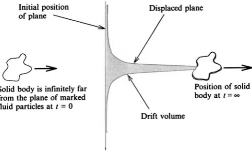
Meteorological Office, Bracknell, Berks RG12 2SZ, UK (Received 27 September 1993 and in revised form 8 April 1994)

A body moves at uniform speed in an unbounded inviscid fluid. Initially, the body is infinitely far upstream of an infinite plane of marked fluid; later, the body moves through and distorts the plane and, finally, the body is infinitely far downstream of the marked plane. Darwin (1953) suggested that the volume between the initial and final positions of the surface of marked fluid (the drift volume) is equal to the volume of fluid associated with the ‘added-mass’ of the body.

We re-examine Darwin’s (1953) concept of drift and, as an illustration, we study flow around a sphere. Two lengthscales are introduced: pmax, the radius of a circular plane of marked particles; and XO, the initial separation of the sphere and plane. Numerical solutions and asymptotic expansions are derived for the horizontal La- grangian displacement of fluid elements. These calculations show that depending on its initial position, the Lagrangian displacement of a fluid element can be either pos- itive - a Lagrangian drift - or negative - a Lagrangian reflux. By contrast, previous

investigators have found only a positive horizontal Lagrangian displacement, because they only considered the case of infinite XO. For finite XO, the volume between the initial and final positions of the plane of marked fluid is defined to be the ‘partial drift volume’, which is calculated using a combination of the numerical solutions and the asymptotic expansions. Our analysis shows that in the limit corresponding to Darwin’s study, namely that both xo and pmax become infinite, the partial drift volume is not well-defined: the ordering of the limit processes is important. This explains the difficulties Darwin and others noted in trying to prove his proposition as a mathematical theorem and indicates practical, as well as theoretical, criteria that must be satisfied for Darwin’s result to hold.

We generalize our results for a sphere by re-considering the general expressions for Lagrangian displacement and partial drift volume. It is shown that there are two contributions to the partial drift volume. The first contribution arises from a reflux of fluid and is related to the momentum of the flow; this part is spread over a large area. It is well-known that evaluating the momentum of an unbounded fluid is problematic since the integrals do not converge; it is this first term which prevented Darwin from proving his proposition as a theorem. The second contribution to the partial drift volume is related to the kinetic energy of the flow caused by the body: this part is Darwin’s concept of drift and is localized near the centreline. Expressions for partial drift volume are generalized for flow around arbitrary-shaped two- and three-dimensional bodies. The partial drift volume is shown to depend on the solid angles the body subtends with the initial and final positions of the plane of marked fluid. This result explains why the proof of Darwin’s proposition depends on the ratio

202

used to illustrate the differences between drift in bounded and unbounded flows. I. Eames, S. E. Belcher and J. C. R. Hunt

An example of drift due to a sphere travelling at the centre of a square channel is

1.

Introduction

When a sphere moves in an unbounded inviscid fluid, one might intuitively expect, as Darwin (1953) remarked, that there would be a net flux of fluid in the opposite direction to the motion of the sphere; a reflux of fluid. Detailed calculations by Darwin (1953) show that there is a volume of fluid that drifts in the same direction as the sphere. This flux of fluid drifting with the sphere can be interpreted as a ‘potential-flow wake’ behind the body.

Darwin (1953) examined the motion of an arbitrarily shaped solid body in an unbounded region of inviscid fluid. The body starts infinitely far from an infinite plane of marked fluid, and travels at a constant speed towards the plane, which is then distorted by the passage of the body. Darwin defined the drft volume to be the volume between the initial and final positions of the surface of marked fluid and suggested that drift volume is equal to the volume of fluid associated with the hydrodynamic mass of the body (figure 1). The hydrodynamic mass of a body is the mass of fluid that must be added to the body when calculating the total kinetic energy; it is commonly referred to as ‘added mass’ (Batchelor 1967, p. 407). Darwin’s proposition is an appealing result and has been further investigated by Lighthill (1956), Yih (1985) and Benjamin (1986).

Darwin’s proposition has been referred to several times as Darwin’s theorem. But it has been pointed out by Darwin himself and by Benjamin (1986) that the drift volume depends critically on the method of evaluation of certain integrals and so the proposition cannot be proved to be a mathematical theorem without delicate qualifications. We therefore prefer the term ‘Darwin’s proposition’.

Darwin’s proposition has been used to interpret measurements of bubble motion and other two-phase flows. For example, Bataille, Lance & Marie (1991) set up an experiment with a lower layer of fluid that was dyed and slightly denser than an upper layer of fluid. Bubbles were released beneath the interface, which was distorted by the passage of a bubble. The volume of fluid that drifted with a bubble was measured and found to be equal to Darwin’s calculation, i.e. half the bubble volume which is equal to the added mass volume of the bubble for potential flow. Interestingly, Rivero’s (1990) numerical calculations of the added-mass volume of accelerating rigid spheres and bubbles in viscous flows (Re w 100) also agree with the volume calculated using potential flow.

Drift, partial d r f t and Darwin’s proposition

Initial position

body at t =

-

Solid body is infinitely far

from the plane of marked fluid particles at t = 0

RGURE 1. Sketch of the drift volume (as defined by Darwin).

203

--.)

plane t = 0

_.--

-

stratification

1

_ _ _ _ _ _ _ _ _ _ _ _ _ _ _ _ _ -

---

* - - - - _ _ _ _ _ _ _ _ _ _ _ _ _ _ _ _ _

...

204

-

-

I. Eames. S. E. Belcher and J. C. R. Hunt

/

-

I

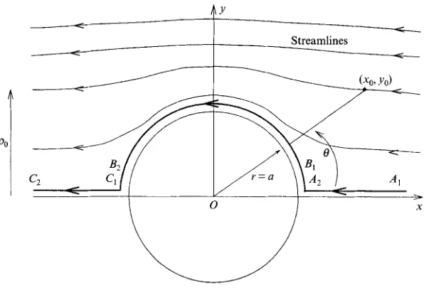
FIGURE 3. Streamlines close to the sphere.

It is shown that, in the configuration studied by Darwin (1953), Yih (1985) and Benjamin (1986) when both xo and pmax are infinite, the problem is not well-posed, because the drift volume is not well-defined. Yih’s procedure does in effect assume as

pmax/xo -+ 0 as xo --+ 00.

In $4 a general expression for horizontal Lagrangian displacement is derived for an arbitary potential fluid flow superimposed on a constant-mean-velocity flow. The partial drift volume is shown to depend on the solid angles subtended by the body and initial and final positions of the plane of marked fluid. This analysis is generalized to arbitrarily shaped two- and three-dimensional bodies.

In $5, we use our results for drift due to a sphere in unbounded flow to indicate how drift in bounded flow can be calculated. The sphere is assumed to travel along the centreline of a square tube. This three-dimensional example can be applied to practical problems (e.g. the experiments of Bataille et al. 1991; Kowe et al. 1988).

Finally it is worth noting that there are an increasing number of practical fluid mechanics problems whose solution depends on having a good estimate of the drift volume (e.g. Kowe et al. 1988). For example, the partial drift volume is also of importance when large particles are ejected into a cloud of smaller particles, or a rising bubble formed in a temperature gradient (figure 2b).

2. Horizontal Lagrangian displacement for flow around a sphere

Consider the inviscid flow caused by a fixed sphere of radius a in a uniform stream of speed -Ux, where U is constant and x is the unit vector parallel to the x-axis. The flow is axisymmetric and so it is sufficient to consider a single (x,y) plane, shown in figure 3. In spherical polar coordinates the velocity potential and streamfunction are

Drift, partial drijit and Darwin's proposition 205 where r is the distance from the origin and 0 is the angle made with the x-axis. The velocity components are

Lighthill's (1956) notation is used, so that a fluid element marked at time t = 0 with

Cartesian coordinates (XO, yo) is advected to the position (-m, PO) as t + co. Equation

(2.lb) is used to relate PO, xo and yo, so that

a3

)

It is more convenient to expresss the position of a marked fluid element at time t in terms of polar coordinates (r(t),e(l)), which is related to its ultimate position by

(2.4) The roots of the cubic equation (2.4) can be found analytically (e.g. Abramowitz &

r3 -

*

- a3 = 0. sin2

e

Stegun 1965, p. 17), and when sin8

>

(4/27)'/6po/a

whereas when sin 8

<

(4/27)'/6po/a

33/2a3 cos a, where cos 3a = - sin3 8.

2Po

r = -

J3

sin

e

2P:

The horizontal Lagrangian displacement of the fluid elements, X , is defined to be

o' _{a3(2 cos2}

e

_{- sin2}

e)

dt. 2r3

X =

loo(

U

+

u,)dt =

1

U

This expression is manipulated using (2.2b) to eliminate dt and (2.4) to remove the r3 term; X is then given by

where 00 = arctan(yo/xo). The horizontal Lagrangian displacement is written in (2.8) as a function of PO, the final vertical position of the marked fluid element, and B0

the initial horizontal position. This choice of variables simplifies the calculation of the partial drift volume in 94. The integral (2.8) cannot be expressed in closed form and approximations are found using asymptotic analysis. Also, the dependence of X(p0,xo) on po is found directly from expression (2.8) rather than using, as Lighthill (1956) did, X = limt+m( Ut

+

x).

2.1. Asymptotic formulae for X(p0, XO) f a r from the centreline

206 I. Eames. S. E. Belcher and J. C. R. Hunt

7 I I I I I I I

(a)

6 - I

I

5 - -

t

4 -

i

4

9

x=

9a6rc

2 - Q 64Yi

Y a

-

?

3 -

+

-

4a 2 ~ 3 " ~

x=

- 3 log

(--)

----_._...____

1 -

I I I I I

0

7

6

5

4

Y a

-

3

2

( 2 3

1

a

Horizontal Lagrangian displacement, Xla

I, I I I I I 1

c

&

x=o

4a 2a33'4 3

x=

- log

(yo

j

----..____.._ .

I I I I ,

Horizontal Lagrangian displacement, Xla

FIGURE 4 (a, b). For caption see facing page.

which is equation (64) in Lighthill (1956). In this approximation, the integral in (2.8) can be evaluated and the horizontal Lagrangian displacement is

a3

X = - [ C O S ~ do - cos

e,]

2P;

1 . 5 13

Drift, partial drift and Darwin’s proposition 207

7

6

5

4

Y

a -

3

2

1

0 I

0 0.02 0.04 0.06 0.08

Horizontal Lagrangian displacement, Xla

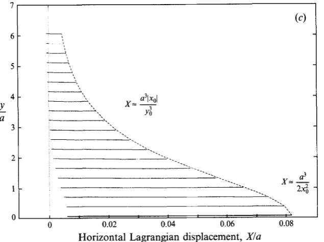
FIGURE 4. Plot of the trajectories of marked fluid particles on planes (a) Xg = 50.0a, ( b ) xg = 2Sa,

(c) xg = -2.5~1.

which expresses the displacement in terms of the initial position, through the 80

dependence, and the final position, through the po dependence. Far from the centreline, yo

+

a so that from (2.3), PO

=

yo and Oo w arctan(po/xo).

We further approximate (2.10) in order tc calculate the horizontal Lagrangian displacement of fluid elements marked far in front of the sphere, when 80 + 0, and

far behind the sphere, when O0 +

x.

When 00 -+ 0 and po/a

+

1, (2.10) gives

9a6x a3

X(p0,xo) = - _64p:

-

- _{2 4} (2.11)

Lighthill (1956) obtained the first term of (2.11) (his equation (67)) when he considered the limit of xo + 00. The new second term arises from xo being finite and gives an important contribution to X . When Oo +

x

and po/a

+

1, (2.10) gives

a3 3a6 _(2.12)

which is independent of po and therefore flat.

The horizontal Lagrangian displacement of a fluid element marked far from the symmetry axis and with xo small is now calculated by allo~ing 80 -+ x/2 in (2.10);

this shows that

(2.13)

208 I. Eames. S.E. Belcher and J. C. R. Hunt

2.5a

= 0.17a

\

eqn (2.16)

No singularity in X eqn (2.18)

Horizontal displacement of the fluid particle has a logarithmic singularity here.

FIGURE 5. Schematic of where the errors of the asymptotic expansions are small.

(2.11) this surface is given approximately by

yo N ( 9 7 3 li5 (2.14)

Finite xo were not analysed by Darwin (1953) or Lighthill (1956): they considered the limit xo + 00

.

Consequently, they found positive horizontal Lagrangian displacement

for all yo (see figure 4a). Equation (2.13) shows that if xo is positive and finite then, far from the centreline, fluid elements are displaced in the direction opposite to the motion of the sphere. This region of negative horizontal displacement, i.e. a region of reflux, is a consequence of introducing a finite xo and has interesting implications for practical purposes. An example of a region of reflux is shown in figure 4(b).

The asymptotic formula (2.10) is used in $3 to evaluate the partial drift volume so it is important to find where this is a good approximation to X . A suitable restriction, obtained from (2.8), is 3a3 sin2 8 < h2p;r. The most restrictive inequality for xo

<

0 is

(2.15)

When _Ixo/ 9 yo, this implies yo

>

f i a 3 / 2 / ~ A / 2 and when 1x01 4 yo it requires yo

>

24/3a. These conditions define two regions that are sketched in figure 5. If xo

>

0, the smallest value of r is rm,n and occurs when 0 = n/2, where

3 3 112 -

rmin (1 - a /rmin) - PO.

A suitable requirement for (2.10) to be a good approximation to X for xo

>

0 is 3a3

<

h2p,?jrmin from which we obtain the requirement PO

>

161/3(15/16)1/2a

=

2.5~.

Lighthill (1956) estimated that the region of convergence for the expansion of X , when p o + a and xo + co, is PO

>

1.5~. We find that when PO

>

2.5a the first two

Drift, partial drift and Darwin’s proposition

2.2. Asymptotic expansions of X(p0, XO) close to the centreline

Lighthill (1956) derived two expressions for X close to the centreline when xo + co:

one along the streamline segment AIA2 and another along B1B2 (see figure 3). These expressions were matched to determine the horizontal Lagrangian displacement. We use a similar approach to calculate X when xo

> a

and po/a ₄ 1, but generalize Lighthill’s (1956) analytical results by analysing finite xo.

209

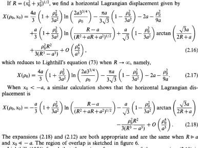
If R = ( x i

+

we find a horizontal Lagrangian displacement given by

3(R3 - a3)

+

(2.16)

which reduces to Lighthill’s equation (73) when R + 00, namely,

(2.17)

When xo

<

-a, a similar calculation shows that the horizontal Lagrangian dis- placement is

- PiR2

+ O

(2).

(2.18)

3(R3 - a3)

The expansions (2.18) and (2.12) are both appropriate and are the same when R b a and xo ₆ - a. The region of overlap is sketched in figure 6.

Lighthill (1956) found that the region of convergence of the expansion (2.18) is

PO

<

0.4~. We find that the horizontal Lagrangian displacement (2.17) can be represented by the first two terms of its asymptotic expansion when PO

<

a$/lO

=

0.17~.

2.3. Numerical calculation of fluid particle trajectories

The asymptotic expansions derived in the previous sections were supplemented with numerical calculations to obtain solutions for horizontal Lagrangian displacement over the whole ranges of xo and PO. Trajectories in the Cartesian coordinate system

were obtained by solving

dx

84

dY -

a4

dt - - ax’ d t

_ -

ay’

- -

-subject to the initial condition x = xo and y = yo at time t = 0.

Figure

4

shows examples of fluid particle trajectories plotted in Cartesian coor- dinates as (X(p0, XO, t), y(p0, xo, t)), together with the deformed marked planes, for xo = 50.0a, 2Sa, -2.5~. The horizontal Lagrangian displacement close to the cen- treline when xo = 50.0~ is approximately the same as when xo -+ 00. If xo + 00

210

2.12

2.10

2.08

2.06

Y

a

- 2.04

2.02

2.00

1.98

I. Eames, S. E. Belcher and J. C . R. Hunt

I I I I A 1 I I I v

I co=o

I

I I

Sweeping motion, 1st term in (2.10)

-

I Drift, 2nd term in (2.10)

I I I I I

-0.04 4 . 0 3 4 . 0 2 4 . 0 1 0 0.01 0.02 0.03 0.04 0.05

Horizontal Lagrangian displacement, Xla

FIGURE 6. Trajectory of a single marked fluid element on the streamline po = 2 . 0 ~ . The diamonds

( 0 ) indicate where marked fluid particles start on the streamline.

When xo + -00, the perturbation to the fluid flow due to the presence of the

sphere is neglible so that the Lagrangian displacement of the marked fluid particles is zero. The fluid particles drift in the same direction as the sphere when xo is large and negative as shown in figure 4c, which uses xo = -2.5~.

The trajectories plotted in figure 4 show two distinct features: a sweeping motion and a drift. Close to the centreline the contribution to X from the positive drift is larger than from the sweeping motion, but far from the centreline the sweeping motion is larger than the drift forwards. Figure 6 shows that the sweeping motion gives a larger contribution than the small drift forwards and that the displacement of the fluid particle depends on where it is initially marked. In $4 we explain how the sweeping motion and the drift give two separate contributions to partial drift volume.

3.

Partial drift volume

The drift volume is defined to be the volume between the initial and final position of the marked plane, i.e. the integral of the drift, X , over the marked plane (Darwin 1953). By analogy, we define the partial drift volume,

D,,

to be the volume between the final and initial positions of a marked plane of finite extent which is initially placed a finite distance from a solid body (see figure 2a). For a circular marked plane that is distorted by a sphere, the partial drift volume is

(3.1)

Drift, partial drift and Darwin’s proposition 21 1

We define D to be the drift volume calculated using Darwin’s method, so that D is the volume of fluid associated with the hydrodynamic mass of the body.

3.1. Asymptotic expression for D, when the marked plane starts far from the sphere

The asymptotic expressions derived in $2 for the drift are now used to find approxi- mations to the partial drift volume. Two limits are treated: firstly, the marked plane starts far upstream of the sphere and, secondly, the plane starts far downstream of the sphere.

Darwin (1953, $2) showed that when xo --+ co and pmaX/xo + 0 the drift volume

is equal to the volume of fluid associated with the hydrodynamic mass of the solid body, e.g. for a sphere D = ;nu3. When xo + 00 and pmax is large but finite, the partial drift volume, D,, is close to D .

If xo + 00 then the partial drift volume, D,, is related to drift volume, D, by

If pmax/a

+

1 , and pmax d XO, then the integral can be evaluated because X can be

approximated by (2.11). The result is that

It is clear from this asymptotic analysis that, when xo +

co

and pmax is finite, D,

is only approximately equal to D . Benjamin (1986) however suggested that, under these conditions, D, is equal to D . Benjamin’s (1986) error can be traced to the manipulation given in going from his equation ( 5 ) to (6).

A second limit is that the marked plane starts far downstream of the sphere, i.e.

xo Q -a. The approximate expression for X given in (2.12) is then valid over the whole range of po and the partial drift volume can be evaluated; it is

This result is surprising because it shows that D, can remain finite if xo and pmax

both become infinite, i.e. no matter how far the plane starts behind the sphere, if pmax

is sufficiently large, the drift volume can have any value. This observation indicates why Darwin’s proposition must be qualified before it can be stated as a theorem.

3.2. Asymptotic expansions for D, when the marked plane is large

If xo d - a then (2.10) is a good approximation to X over all po and the partial drift volume can be evaluated :

When xo

+

a and p o / a

+

1, (2.10) is approximately equal to

a3 2Po

~ ( p o , xo)

-

lim ~ ( p o , xo)

+

[ C O S ~ 60 - cos

e,].

xg+m

212

- DP D

I. Eames, S . E. Belcher and J. C . R. Hunt

1.2 I . I ’ I ’

-0.6 I I . I . I . I . I

0.001 0.01 0.1 1 10 100

PmaxllXol

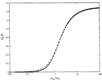
FIGURE 7. Normalized partial drift volume ( D , / D ) plotted against prnax/lx~I for: 0, xo = 500.0~;

+,

xo = 50.0a; and 0, xo = 10.0~. Equation (3.9) is plotted as _.

when po/a 4 1. Thc second terms of the right-hand sides of (3.6) and (3.7) are due to introducing finite XO, and they asymptotically match when x0 .+. co. This leads to the

suggestion that

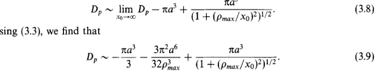
Using (3.3), we find that

(3.9)

Below, we find a good agreement of (3.9) with the numerically calculated value of D,

for a large range of P m a x / X o .

3.2.1. Numerical calculation of partial d r f t volume

Long computational times are required to follow the large numbers of marked fluid particles needed to evaluate D , and so we used the asymptotic expansions of X(p0, XO) where they are good approximations. Consequently, when xo

>

a, X ( p 0 , XO)

was calculated numerically only in the range 0.1

d

po/a

<

4.0. Equation (2.10) was used to approximate X when po/a

>

4.0 and (2.16) when po/a

<

0.1. When xo

<

-a,

the horizontal Lagrangian displacement is evaluated using (2.10) for po/a > 4.0 and numerically when po/a

<

4.0.

D r f t , partial d r f t and Darwin’s proposition 213

1.6 I I

I

Pmax~lXOl

FIGURE 8. Normalized partial drift volume ( D , / D ) plotted against p m a X / l x ~ l for: 0, xo = -10.0~;

+,

xo = -4.0a; and 0, xo = -1.0~. Equation (3.5) is plotted as _.

pmax/xo d 1, D,/D -+ 1; by contrast when pmax/x0

+

1, D,/D -+

-$.

The asymptotic

expressions for Dp(pmax, XO) are also plotted for comparision.

The curves in figures 7 and 8 show that when xo becomes large, D p / D asymptotes to a function of pmax/xo. When both XO and pmax become infinite (the case studied

by Darwin 1953 and Benjamin 1986) our calculations show clearly that the value of

D , / D depends on how the double limit is approached. First taking xo -+

kco

and

then pmax -+ co is equivalent to

lim lirn Dp(pmax,x0) = lim Dp(Pmax, XO),

Pmax+m xo+fm Pmox 1x0 +!dl

whereas first taking po + 00 and then XO -+

+co

implies

lim lirn Dp(pmax,x0) = lim Dp(Pmax, XO).

xo++m Pmax+m Pmax 1x0 ++x

Figures 7 and 8 show that the partial drift volume asymptotes to different values in these two limits. Hence the drift volumes as calculated by Darwin (1953) and Benjamin (1986) require careful definitions and therefore cautious use in experiments! We are able to state Darwin’s result as a theorem: when a solid body passes through a large

214

4. General analysis

Our detailed analysis of drift and partial drift volume for flow around a sphere shows several interesting features which we now generalize to bodies of arbitrary shape.

I. Eames, S. E. Belcher and J. C . R. Hunt

4.1. General expression for the horizontal Lagrangian displacement

In $2 it was shown that horizontal Lagrangian displacement can be positive - a drift - or negative - a reflux. A general analysis is now developed to explore the processes

that cause the displacement.

For potential flow around an arbitrarily shaped body fixed in a uniform stream of speed - U x , the horizontal Lagrangian displacement is

.I'

(4.1)

1

X =

s

( U

+

u,)dt = -

/

u ( ~ , U

+

u2)dt

+

g 2 d t ,

where q = {(U

+

u , ) ~

+

us

+

u:)"~, the fluid particle speed is v = (u2

+

us

+

u:)'I2

and ux,uy, u, are the velocity components of the fluid relative to the body. Two results from potential flow theory, namely (Yih 1985)

are needed to manipulate (4.1) into

(4.2a, b)

The first integral can be evaluated; it is

h 1

lo

{

u

(

$)v,*

+

1) d 4 =

[

$

+ X I 4 0 @'

Yl") 1 z l v ) 1

-(U

+

u,)dx

+

lo

p y d y

+

lo

UU&. (4.4)

Hence X(x0, yo, 20, t) is given by

+

.I'

;q2dt. (4-5)

W x o , Yo, ZO, t) = - -( U

+

u,)dx -

Here xl(t) = xo - Ut +X(xo,yo, t), yl(t) and zl(t) are the Cartesian coordinates of the fluid element at time t.

Assuming in the far field that the flow due to the solid body can be approximated by a dipole of strength $Ua3, then far from the centreline (so that yo 9 xo

+

a) the

first term in (4.5) is O( Ua3/r2) and dominates the other terms, which are O( Ua6/r5). The horizontal Lagrangian displacement is therefore given approximately by

Drift, partial drift and Darwin’s proposition 215 If a fluid particle starts close to the centreline, so that yo Q a and xo %yo, the first

term in (4.5) is O( Ua3/r2), as in the previous paragraph. Such particles travel close to the stagnation points on the body, where they have high residence time. Hence these particles will be displaced a large distance forward. Therefore the last term in (4.5) dominates and the horizontal Lagrangian displacement is approximately

which is the total kinetic energy along a streamline per unit area normal to the direction of motion of the sphere. Expression (4.7) represents the drift of marked fluid with the body and is approximately equal to the second term in (2.10).

4.2. Interpretation of D,

The horizontal Lagrangian displacement given by (4.4) and (4.5) is now used to evaluate the partial drift volume. The fluid flow due to the motion of a sphere is equivalent to the flow due to a dipole. Furthermore the far-field flow due to an arbitrary solid body is that of a dipole (Batchelor 1967, p. 399). The partial drift volume due to an arbitrary body may be approximated by studying flow around a sphere.

Consider a marked plane SO whose perimeter is Bo in the (y,z)-plane a distance xo from the sphere and let R be the radius of the largest circle centred on the x-axis which lies within SO. The notation is shown in figure 9. The marked plane is distorted by the sphere to give a surface S,, whose perimeter is Bt. Let S be the projection of S,

onto the (y, z)-plane, i.e. S is also bounded by Bt, but lies entirely in the (y, z)-plane. Also, V t is the volume bounded by the surfaces St, SO and the surface generated as the perimeter B, is advected along. Let V be the volume enclosed by the surfaces S ,

So and the surface traced by Bt.

For flow around a sphere, when the velocity potential is given by (2.la), the general expression (4.5) becomes

where A = $Ua3 is the dipole strength of the sphere. The partial drift volume for the sphere is

By definition, the solid angle subtended by So to the centre of the sphere is

while the solid angle subtended by S to the centre of the sphere is

as =

-b

Y d S .

(4.10)

(4.11)

216

I.

Eames. S. E. Belcher and J. C . R. Hunt

SO

FIGURE 9. Notation for the distortion of an arbitrary-shaped plane by a sphere.

can be shown that (see Appendix)

Substituting the approximations (4.12 a,b,c) into (4.9), we find that the partial drift volume can be written in terms of the solid angles subtended by the marked plane to the centre of the sphere at its initial and final positions:

(4.13)

Drijit, partial drijit and Darwin's proposition 217 term in the expression for partial drift volume means that the partial drift volume is also non-absolutely convergent when pmax + oc, and xo + co. The second term is the volume through B, associated with the kinetic energy of the fluid in Y due to the presence of the body. The second term is positive and represents a volume of fluid drifting with the body.

When the sphere lies within V the last term is approximately CMV, the volume of fluid associated with the hydrodynamic mass of the solid body, where CM is the added-mass coefficient of the sphere and V is its volume. Whereas, if the sphere does not lie within Y , then the last term in (4.13) is neglible. Therefore, provided the sphere passes through the marked plane

(4.14)

A

D,

-

-- ( 0 s

+

a&)

+

CM V .

This equation is exact when xo + 00, R + 00 and t + co.

We can generalize (4.14) to flow around an arbitrarily shaped three-dimensional solid body. Consider separately the contributions to reflux from outside and inside a circular plane of radius b. Outside this circle, the flow disturbance due to the body is at leading order equivalent to a collection of dipoles of total strength A.

The generalization of (4.14) to an arbitrary body then relies on showing that, if the marked plane is sufficiently large and far away, then the contribution to reflux from the circle is small. The partial drift volume is given by

A

D,

-

-- (Ws+Wso)+O

(

+xb2

(-$

+

$))

+l

[

$

+

x]' 2xydy+CMV. (4.15)

U

0

Here the sum of the first two terms is the reflux due to the dipole outside the circle; the third is the reflux inside the circle; and the fourth is the volume drifting with the body. The third term is of

when 1x0 - Utl % b and 1x01 % b. In the far field, the velocity potential is that of a

dipole so that the third term is

+

4))

0

(

$xb2

(

(xo - Ut)2 xo

1

Therefore, when the plane is much larger than the circle, i.e. R % b, and the initial and

final position of the marked plane is far from the solid body, (4.14) holds.

Similarly, partial drift area for flow around two-dimensional bodies can be expressed as

A

D,

-

-- U (a,

+

ao)

+

CMV, (4.16)

where @,,a0 are the angles subtended by the line of marked particles to the centre

of the solid body, A the equivalent strength of the dipoles and CMV area of fluid associated with the hydrodynamic mass of the body.

5.

An

example of drift in bounded

flow

218 I. Eames, S. E. Belcher and J. C. R. Hunt

Initial position of marked plane

b

I

/'

Enhanced

-

reflux

a3

b2

FIGURE 10. An example of partial drift in bounded flow. (a) Notation, ( b ) reflux of fluid is shown when xo -+ a. A comparison with unbounded flow is shown.

of the volume of the solid body (Darwin 1953). Darwin 1953 discussed bounded flow, stating that there are two contributions to the partial drift volume: a volume of fluid drifting with the body and a reflux volume which is spread across the cross-section of bounded flow. He illustrated these effects using the two-dimensional example of the drift due to a cylinder moving between two solid planes. We now use our results to discuss the distortion of a marked plane by a sphere travelling along the centreline of a long square tube of side b, whose dimensions are much larger than the radius of the sphere, a. The notation is shown in figure 10. This example is interesting in light of the experiments of Bataille et al. (1991).

Drift, partial drift and Darwin’s proposition 219

0 0 0 0

, , 0 ,’

I

, I

I

l

I _, ,

\

0 ’\ 0

\ , \

0 ’\ 0 _{Dipoles within a distance}

xo from the sphere contribute to the reflux

I

!

-3- I

Y I

l

- b -

0 0

Sphere ,I

, 0 ,!‘ 0

2

I

Image dipoles of strength fa3U pointing of the page

FIGURE 11. The distribution of image dipoles required to satisfy the kinematic condition on the sides of the tube.

boundary condition on the sphere is satisfied by introducing additional dipoles of strength O( $a3Ua3/b3), which are neglible when b % a. The velocity potential is a linear combination of the potentials due to all these dipoles, so that

X

4

-

-UX - 4ua3 (1

+

o(a3/b3))

2

(x2

+

(y

+

ib)2

+

( z

+

jb)2)3/2’ (5.1) ij=-a0

where i , j are integers.

The volume of fluid drifting with a sphere in bounded flow is the same as for unbounded flow except for the modificaiton due to image dipoles. The fluid drifting with the sphere is 4nA/U-V (Taylor 1928), where A is the total dipole strength within the sphere and V the volume of the sphere. Now A = ;a3U(l

+

O(a3/b3)), where the O(a3/b3) corrections are from the image dipoles used to satisfy the kinematic boundary condition on the sphere surface. The fluid drifting with the sphere in bounded flow therefore approaches that of unbounded flow when b

+

a.

However, the reflux in bounded flow differs substantially from unbounded flow -

this can be shown by calculating the negative Lagrangian displacement of a marked plane initially far in front of the sphere. The distribution of reflux across the cross- section of the tube depends on the ratio b/xo. The negative Lagrangian displacement of a marked fluid element is [ 4 / U

+

XI:;

(from (4.3) and (4.4)). Substituting the velocity potential (5.1), we find that the negative displacement of the particle, Xneg, is approximately

X

220

If XI -+ -00 and xo

+

b, the negative Lagrangian displacement is

I. Ea,mes, S. E. Belcher and J. C. R. Hunt

a) _u3Tt

b2 - -

XO

(xi

+

( y

+

ib)2

+

( z

+

jb)2)3/2

xneg

-

-La3

.

t,J=--oo

a3n

b2

’

- -

1 a3 1

2 x i , - -

- _ _

(1

+

(y

+

i b / ~ ~ ) ~

+

( 2

+

j b / ~ ~ ) ~ ) ~ / ~ rJ=-m

where

7

= y / x o and 2 = x/x0. The quantity summed over i and j is 0(1) for lil,ljl 6 xo/b. There are O(nxt/b2) combinations of i and j for which lil,ljl

<

xo/b,

so that

As xo -+ 00, the negative displacement of a marked particle in bounded flow is

therefore independent of xo and constant across the tube. Therefore, as xo -+ co the

reflux is spread uniformly across the tube, agreeing with Benjamin (1986). By contrast reflux in unbounded flow is dependent on xo and spread uniformly within a distance

XO from the centreline (figure 4b).

The negative Lagrangian displacement of the marked plane can be calculated exactly when xo -+ 00. The reflux volume is equal to

D,

- CMM, from (4.14). But the

drift volume is equal to -V, where I/ is the volume of the sphere, so that the reflux volume is -(1

+

CM)V = - h a 3 . In the previous paragraph, we showed that when xo -+ 00, reflux is spread uniformly across the tube, so that the negative displacement

of the marked plane is -2na3/b2, since the cross-sectional area of the tube is b2. It is important to note that though the negative displacement -2na3/b2 is a small quantity, reflux volume, which equals - h a 3 , is not.

When a Q xo

a

b, the reflux of the fluid can be examined qualitatively by studying the contribution to reflux from a single image dipole close to the tube wall. Figure 12 shows the separate contribution to reflux from the image dipole and sphere, and also the combined contribution. We see that the presence of the boundary enhances reflux and that there is a significant variation of reflux within a distance O(b/2 - XO)

of the boundaries.

When b

-

a, more (positive) image dipoles are required within the sphere and hence the volume of fluid associated with the hydrodynamic mass, D = 4nA/U - I/ (Taylor 1928), increases. The volume of fluid drifting with the sphere therefore increases. Since the flow is bounded, partial drift volume is constant and the reflux volume decreases, i.e. becomes more negative.

6. Conclusion

We have calculated asymptotic expressions for horizontal Lagrangian displacement, X , of a marked fluid element due to the motion of a sphere. Far from the centreline it was shown that X

<

0 for certain finite values of XO, which is in contrast to previous investigations that predicted X

>

0 for infinite XO. The partial drift volume

Drft, partial d r f t and Darwin’s proposition

Image dipole

/

22 1

...

J

Reflux due to ... 3-

image dipole \. ...

‘

Reflux due to sphere za3

moving to x , = - 00 is -

b2

Enhanced reflux near boundary

...

Reflux due to isolated sphere

\..

l

t’;

Sphere in tube

iitial position of

marked plane

b

FIGURE 12. The separate contributions to the reflux from the sphere and nearest image dipole are shown for a 4 xo 4 b. The total reflux varies significantly close to the tube walls.

A general expression has been derived for the horizontal Lagrangian displacement of a fluid particle due to an arbitrary potential flow superimposed on a constant velocity. The displacement is the sum of two contributions: a drift forward and a reflux backwards. This new expression for Lagrangian displacement was used to calculate the partial drift volume due to a sphere and it was shown that there are two contributions to the partial drift volume. One is the volume associated with the kinetic energy of a region of the fluid and was obtained by Darwin. The second new contribution is the volume associated with the momentum of a region of the fluid, which is proportional to the sum of the solid angles subtended to the centre of the sphere by the marked plane at its initial and final positions. This expression for the partial drift volume could be generalized to arbitrary three-dimensional solid bodies because they have a dipole flow in the far field.

An example of drift due to a sphere in flow bounded by a square tube was given illustrating differences between bounded and unbounded flows. The reflux volume was shown to depend on the initial separation of the marked plane compared with the width of the tube. This example has practical applications.

We are now using the concept of partial drift volume to examine how dust is entrained in the wake of a sand particle as it leaves the ground by calculating the distortion of a plane of marked particles by a sphere moving away from a solid boundary.

I.E. was supported by the Science and Engineering Research Council, under a CASE award with British Nuclear Fuels. S.E.B. gratefully acknowledges the financial support of the National Environmental Research Council under grant GR317886. We

222

I.

Eames, S. E. Belcher and J. C. R. Hunt

are grateful for helpful conversations with Dr G. Duursma and Dr J.R. Ockendon concerning bubbles in bounded flow.

Appendix

To show (4.12a), we first note that the streamfunction, y , is related to po by

y = - i p i U so that dy, = -Upodpo. The streamfunctions for three-dimensional flows are denoted by y and

x

(Yih 1985). Using ( 4 . 2 ~ ) we find that

where d V is a volume element. Therefore

When the sphere has passed far through the marked plane, the second integral is

O ( U ~ / X ’ ~ ) , whereas if the sphere has not passed through the plane the second integral is O ( U * / X ’ ~ log(a/Ix’I)), where x’ = xo - Ut. In either case, under the assumption of

lx’l 9 a, the approximation (4.12~) is valid.

To show (4.12b), we transform the area elements on S to the elements on SO using (2.3). Thus,

Y d Y t = YodYo

3y;a3

l+x

1 +3a3y: 7

(

1 + - -

;;E)

2rt

Each position of an area element in the S-plane can be described by cylindrical coordinates (yt, rp), where cp is the angle the element made the (x, y)-plane. Since there is no rotational drift dS, = ytdytdrp and dSo = yodyodq. Therefore,

3a3

(

siyiOo sin2 8, sin Ot cos 8, dX Y d S =

Lo

- cos

eo

d S o + i o

i(----

r

:

r, d Y t ) dSo

6

₁

₊

_{3a3 2rt3 sin2 ‘t (1}

₊

_cot

_B,dX))

_{dY t}

(A 4) The second term in (A4) is at most O(a2/lx’l,a2/lxol) and small when Jx’I 9 a and

Equation (4.12~) is derived by using the cosine rule and simple geometrical relations

lxol 9 a, so that approximation (4.12b) is valid.

shown in figure 9. We find

Drift, partial drift and Darwin’s proposition

REFERENCES

ABRAMOWITZ, M. & STEGUN, I. A. 1965 Handbook of Mathematical Functions. Dover.

BATAILLE, J., LANCE, M. & MARIE, J.L. 1991 Some aspects of the modelling of bubbly flows. In

Phase-Interface Phenomena in Multiphase Flow (ed. G.F. Hewitt, F. Mayinger & J.R. Riznic),

223

pp. 179-193.

BATCHELOR, G. K. 1967 An Introduction to Fluid Dynamics. Cambridge University Press. BENJAMIN, T. B. 1986 Note on added mass and drift. J. Fluid Mech. 169, 251-256. DARWIN, C. 1953 Note on hydrodynamics. Proc. Camb. Phil. SOC. 49, 342-354.

KOWE, R., HUNT, J. C. R., HUNT, A., COUET, B. & BRADBURY, L. J. S. 1988 The effects of bubbles on the volume fluxes and the presence of pressure gradients in unsteady and non-uniform flow of liquids. Intl J. Multiphase Flow 14, 587-606.

LAMB, H. 1932 Hydrodynamics. Cambridge University Press.

LIGHTHILL, M. J. 1956 Drift. J. Fluid Mech. 1, 31-54 (and Corrigendum 2, 311-312).

RIVERO, M. 1990 Etude par simulation numkrique des forces exercees sur une inculsion sphkrique par un Ccoulement accC1CrC. PhD thesis, Institute de MCcanique des Fluides de Toulouse, Toulouse.

TAYLOR, G. I. 1928 The energy of a body moving in an infinite fluid, with an application to airships.

Proc. R. SOC. Lond. A 70, 13-21.

WEODORSEN, T. 1941 Impulse and momentum in an infinite fluid. Von Khrmcin Anniversary Volume,

pp. 49-58. California Institute of Technology.

YIH, C.-S. 1985 New derivations of Darwin’s theorem. J. Fluid Mech. 152, 163-172.