Available Online atwww.ijcsmc.com
International Journal of Computer Science and Mobile Computing
A Monthly Journal of Computer Science and Information Technology
ISSN 2320–088X
IMPACT FACTOR: 5.258IJCSMC, Vol. 5, Issue. 7, July 2016, pg.225 – 233
DIGITAL IMAGE
RESTORATION BY USING THE
JOINT STATISTICAL MODEL
ABSTRACT:
This paper presents a completely unique strategy for accurate image restoration by characterizing each native smoothness and nonlocal self-similarity of natural pictures during a unified statistical manner. The most contributions area unit three-fold. First, from the angle of image statistics, a joint statistical modeling (JSM) in an accommodative hybrid space-transform domain is established, that offers a strong} mechanism of mixing native smoothness and nonlocal self-similarity at the same time to make sure a lot of reliable and robust estimation. Second, a replacement variety of minimization purposeful for finding the image inverse drawback is developed using JSM underneath a regularization-based framework. Finally, so as to form JSM tractable and robust, a replacement Split Bregman-based algorithmic program is developed to expeditiously solve the on top of severely underdetermined inverse drawback associated with theoretical proof of convergence. Intensive experiments on image inpainting, image deblurring, and mixed mathematician and salt-and pepper noise removal applications verify the effectiveness of the proposed algorithmic program1.1
Introduction
Images are produced to record or display useful information. Due to imperfections in the imaging and capturing process, however, the recorded image invariably represents a degraded version of the original scene. The undoing of these imperfections is crucial to many of the subsequent image processing tasks. There exists a wide range of different degradations that need to be taken into account, covering for instance noise, geometrical degradations (pin cushion distortion), illumination and color imperfections, inpainting, and blur.
As a fundamental problem in the field of image processing, image restoration has been extensively studied. Image Restoration is the operation of taking a corrupted/noisy image and estimating the clean original image. Corruption may come in many forms such as motion blur, noise, and camera misfocus. It means that to
Damera Divya Rani
M.Tech, PG Student
[email protected]
D. Mahesh Kumar
Associate Professor
reconstruct the original high quality image f(x,y) from its degraded observed version g(x,y) it can be generally formulated as
g(x,y)=H[f(x,y)]+n(x,y)
where H is a matrix representing a non invertible linear degradation operator, n is a usually additive Gaussian white noise. When H is identity, the problem becomes image denoising. When H is a blur operator the problem becomes image deblurring. when H is a mask, that is H is a diagonal matrix whose diagonal entries are either 1 or 0 keeping or killing the corresponding pixels, the problem becomes image inpainting. In this project am focus on image inpainting ,image deblurring and image denoising.
1.2 Aim of the project
The main aim of this project is to produce original high quality image from high-fidelity image restoration by characterizing both local smoothness and nonlocal self-similarity of natural images in a unified statistical manner.
1.3 Methodology
The main contributions are three-fold. First, from the perspective of image statistics, a joint statistical modeling (JSM) in an adaptive hybrid space-transform domain is established, which offers a powerful mechanism of combining local smoothness and nonlocal self-similarity simultaneously to ensure a more reliable and robust estimation. Second, a new form of minimization functional for solving the image inverse problem is formulated using JSM under a regularization-based framework. Finally, in order to make JSM tractable and robust, a new Split Bregman-based algorithm is developed to efficiently solve the above severely underdetermined inverse problem associated with theoretical proof of convergence. These two properties from the perspective of image statistics and propose a JSM for high fidelity of image restoration in an adaptive hybrid space transform domain. Specifically, JSM is established by merging two complementary models: 1) local statistical modeling (LSM) and 2) nonlocal statistical modeling (NLSM).
2. LITERATURE REVIEW
2.1 Introduction
One of the related areas that has seen a recent surge of interest is the area of image processing. With the rise of digital cameras, scanners, and digital imagery, it is more important than ever to have good methods for processing this imagery. The digital images could be distorted or have noise which needs to be removed. Some researchers are interested in recovering important features contained in the image. For example, they may want to recover the location of buildings in satellite imagery or identify objects that are blocking a path for a mobile robot. Given that many images require massive amounts of storage space, we need to consider methods by which to compress the imagery in order to save on storage costs.
A good example of the problems encountered with digital imagery is given by NASA’s Deep Impact mission spacecraft. This satellite was sent to study the innards of a comet, but one of the instrument cameras was not properly calibrated before it was sent into space. The result was all the imagery returned to earth was blurry and all the images would have to be corrected after the data was returned.
In image restoration, a distorted image is restored to its’ original form. This distortion is typically caused by noise in transmission, lens calibration, motion of the camera, or age of the original source of the image.
2.2 Existing Image Restoration Algorithms
It has been widely recognized that image prior knowledge plays a critical role in the performance of image restoration algorithms. Therefore, designing effective regularization terms to reflect the image priors is at the core of image restoration.
Classical regularization terms utilize local structural patterns and are built on the assumption that images are locally smooth except at the edges. Some representative works in the literature are the total variation (TV), half quadrature formulation and Mumford-Shah (MS) models.
2.2.1 Total Variation (TV)
removes unwanted detail whilst preserving important details such as edges. The concept was pioneered by Rudin et al. in 1992.
This noise removal technique has advantages over simple techniques such as linear smoothing or median filtering which reduce noise but at the same time smooth away edges to a greater or lesser degree. By contrast, total variation denoising is remarkably effective at simultaneously preserving edges while smoothing away noise in flat regions, even at low signal-to-noise ratios.
The derivation of a simple algorithm for signal denoising (filtering) based on total variation (TV). Total variation based filtering was introduced by Rudin, Osher, and Fatemi. TV denoising is an effective filtering method for recovering piecewise-constant signals. Many algorithms have been proposed to implement total variation filtering. The one described in these notes is by Chambolle. Although the algorithm can be derived in several different ways, the derivation presented here is based on descriptions given. The derivation is based on the min-max property and the majorization-minimization procedure. Total variation is often used for image filtering and restoration, however, to simplify the presentation of the TV filtering algorithm these notes concentrate on one-dimensional signal filtering only. In addition, the algorithm described here may converge slowly for some problems.
Total variation can be seen as a non-negative real-valued functional defined on the space of real-valued functions (for the case of functions of one variable) or on the space of integrable functions (for the case of functions of several variables). As a functional, total variation finds applications in several branches of mathematics and engineering, like optimal control, numerical analysis, and calculus of variations, where the solution to a certain problem has to minimize its value.
2.2.2 Mumford-Shah (MS) model
The Mumford–Shah model is a functional that is used to establish an optimality criterion for segmenting an image into sub-regions. An image is modeled as a piecewise-smooth function. The functional penalizes the distance between the model and the input image, the lack of smoothness of the model within the sub-regions, and the length of the boundaries of the sub-regions. By minimizing the functional one may compute the best image segmentation. Image segmentation is a hot topic of research given its applicability as a pre-processing technique in many image understanding applications. This Mumford–Shah model describes the image segmentation. The mathematical framework and the main features of the model are sketched along with the procedure leading from the analytical expression of the model to its practical implementation.
The Mumford–Shah functional consists of three weighted terms, the interaction of which assures that the three conditions of adherence to the data, smoothing, and discontinuity detection are met at once. The solution of the Mumford–Shah variational problem is twofold. On one side, a smooth approximation of the data is built so that the data discontinuities are explicitly preserved from being smoothed. On the other side, the model directly produces an image of the detected discontinuities.
An open source software has been developed and used to perform a set of tests on synthetic and real images to demonstrate the feasibility and the effectiveness of the implementation and to give practical evidence of some theoretically foreseen properties of the model. The effect of varying the values of the weight parameters appearing in the Mumford–Shah model has been investigated. In this work, a maximum-likelihood based classifier has been concatenated to the Mumford–Shah model for the processing of a high-resolution photo. The classified image has been compared against the output of the same classifier applied directly to the original photo.
2.2.3 Half quadrature formulation
Half quadrature formulation is a method for numerical integration, or "quadrature", that are based on an expansion of the integrand in terms of Chebyshev polynomials. Equivalently, they employ a change of variables x = \cos \theta and use a discrete cosine transform (DCT) approximation for the cosine series. Besides having fast-converging accuracy comparable to Gaussian quadrature rules, Clenshaw–Curtis quadrature naturally leads to nested quadrature rules (where different accuracy orders share points), which is important for both adaptive quadrature and multidimensional quadrature (cubature).
precomputed, and this computation can be performed in O(N \log N) time by means of fast Fourier transform-related algorithms for the DCT
The classic method of Gaussian quadrature evaluates the integrand at N+1 points and is constructed to exactly integrate polynomials up to degree 2N+1. In contrast, Clenshaw–Curtis quadrature, above, evaluates the integrand at N+1 points and exactly integrates polynomials only up to degree N. It may seem, therefore, that Clenshaw–Curtis is intrinsically worse than Gaussian quadrature, but in reality this does not seem to be the case.
In practice, several authors have observed that Clenshaw–Curtis can have accuracy comparable to that of Gaussian quadrature for the same number of points. This is possible because most numeric integrands are not polynomials (especially since polynomials can be integrated analytically), and approximation of many functions in terms of Chebyshev polynomials converges rapidly. In fact, recent theoretical results[7] argue that both Gaussian and Clenshaw–Curtis quadrature have error bounded by O([2N]^{-k}/k) for a k-times differentiable integrand.
3. Proposed Joint Statistical Modeling in a Space-Transform Domain
The ill-posed nature of image inverse problems, prior knowledge about natural images is usually employed, namely image properties, which essentially play a key role in achieving high-quality images two types of popular image properties are considered, namely local smoothness and nonlocal self-similarity, as illustrated by below figure.
Fig 3.1 Illustrations for local smoothness and nonlocal self-similarity of natural image
The former type describes the piecewise smoothness within local region, as shown by circular regions, while the latter one depicts the repetitiveness of the textures or structures in globally positioned image patches, as shown by block regions with the same color. The challenge is how to characterize and formulate these two image properties mathematically. Note that different formulations of these two properties will lead to different results. Characterize these two properties from the perspective of image statistics and propose a JSM for high fidelity of image restoration in an adaptive hybrid space-transform domain.
Specifically, JSM is established by merging two complementary models: 1) local statistical modeling (LSM) in 2D space domain and
2) nonlocal statistical modeling (NLSM) in 3D transform domain, that is
where τ, λ are regularization parameters, which control the tradeoff between two competing statistical terms. Ψ
LSM corresponds to the above local smoothness prior and keeps image local consistency, suppressing noise effectively, while Ψ NLSM corresponds to the above nonlocal self-similarity prior and maintains image nonlocal consistency, retaining the sharpness and edges effectually. More details on how to design JSM to characterize the above two properties will be provided below.
3.2.Local Statistical Modeling for Smoothness in Space Domain
domain. From the view of statistics, a natural image is preferred when its responses for a set of high passing filters are as small as possible which intuitively implies that images are locally smooth and their derivatives are close to zero.
In practice, the widely used filters are vertical and horizontal finite difference operators, denoted by Dv = [1 − 1]T and Dh = [1 − 1], respectively. Fig. 4.2 shows the gradient picture in horizontal direction of image
Lena and its histogram. It is obvious to see that the distribution is very sharp and most pixels values are near zero. In literatures, the marginal statistics of outputs of the above two filters are usually modeled by generalized Gaussian distribution (GGD). choose Laplacian distribution to model the marginal distributions of gradients of natural images by making a tradeoff between modeling the image statistics accurately and being able to solve the ensuing optimization problem efficiently. Thus, let D = [Dv;Dh] and set v to be to obtain LSM in space domain at pixel level, with corresponding regularization term Ψ LSM denoted by
which clearly indicates that the formulation is convex and facilitates the theoretical analysis.
Fig. 3.2 Illustrations for local statistical modeling for smoothness in the space domain at pixel level.
(a) Gradient picture in horizontal direction of image Lena. (b) Distribution of horizontal gradient picture of
Lena, i.e., histogram of (a).
Note that Ψ LSM has the same expression as anisotropic TV defined and can be regarded as a statistical interpretation of anisotropic TV. It is important to emphasize that local statistical modeling is only used for characterizing the property of image smoothness. The regularization term has the advantages of convex optimization and low computational complexity. There is no need to design a very complex regularization term, since the task of retaining the sharp edges and recovering the fine textures will be accomplished by the following nonlocal statistical modeling.
4.1 Nonlocal Statistical Modeling for Self-Similarity in Transform Domain
Besides local smoothness, nonlocal self-similarity is another significant property of natural images. It characterizes the repetitiveness of the textures or structures embodied by natural images within nonlocal area, which can be used for retaining the sharpness and edges effectually to maintain image nonlocal consistency. However, the traditional nonlocal regularization terms as mentioned above essentially adopt a weighted manner to characterize self-similarity by introducing nonlocal graph according to the degree of similarity among similar blocks, which often fail to recover finer image textures and more accurate structures.
Recently, quite impressive results have been achieved in image and video denoising by conducting the operation of transforming a 3D array of similar patches and shrinking the coefficients It is worth emphasizing that Dabov did excellent work in the image restoration field, especially their famous BM3D methods for image denoising and deblurring applications, which have achieved great success. Our proposed statistical modeling for self similarity is inspired by their success and significantly depends on their work. In this paper, we mathematically characterize the nonlocal self-similarity for natural images by means of the distributions of the transform coefficients, which are achieved by transforming the 3D array generated by stacking similar image patches. Accordingly, this type of model can be named as NLSM for self-similarity in 3D transform domain.
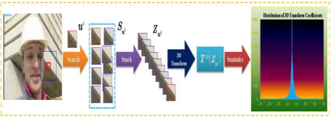
quite efficient (see Theorem 2). Define Sui the set including the c best matched blocks to ui in the searching window with size of L × L, that is, Sui = {Sui⊗1, Sui⊗2, ..., Sui⊗c}. Third, as to each Sui , stack the c blocks belonging to Sui into a 3D array, which is denoted by Zui . Fourth, denote T 3D as the operator of an orthogonal 3D transform and T 3D(Zui ) as the transform coefficients for Zui . Let u be the column vector of all the transform coefficients of image u with size K = bs ∗ c ∗ n built from all the T 3D(Zui ) arranged in the lexicographic order. Note that the orthogonality of 3D transform is momentous in solving NLSM, which will be discussed in the next section. Finally, we analyze the histogram of the transform coefficients, as shown in Fig. 3, which statistically demonstrates that the histogram is quite sharp, and the vast majority of coefficients are concentrated near the zero value.
This is similar to the previous local modeling of images and is also very suitable to be characterized by GGD. Analogous to LSM in space domain, by making a tradeoff between accurate modeling and efficient solving, in this paper the distribution of Θu is modeled by Laplacian function.
Fig. 4.1 Illustrations for nonlocal statistical modeling for self-similarity in 3D transform domain at block level.
Therefore, the mathematical formulation of nonlocal statistical modeling for self-similarity in 3D transform domain is written as
Accordingly, the inverse operator Ω NLSM corresponding to ΨNLSM can be defined in the following procedures. After obtaining Θu, split it into n 3D arrays of 3D transform coefficients, which are then inverted to generate estimates for each block in the 3D array. The block-wise estimates are returned to their original positions and the final image estimate is achieved by averaging all of the above block-wise estimates.
The difference between the proposed NLSM and BM3D method mainly has three aspects. First, we mathematically characterize the nonlocal self-similarity for natural images by means of the distributions of the transform coefficients, which are achieved by transforming the 3D array generated by stacking similar image blocks. Second, for each block, we utilize a fixed number of blocks that are most similar to it within the search window to construct its 3D array. Nonetheless, in the BM3D works many tunable thresholds to choose similar blocks are exploited, which is a bit complicated. Our choice with a fixed number is not only simple but also robust to the similarity criterion. Moreover, the fixed size of each 3D array enables solving the subproblem associated with NLSM quite efficient . Third, the proposed NLSM is more general and can be directly incorporated into the regularization framework for image inverse problems, such as image in-painting, image de-blurring, and mixed Gaussian plus impulse noise removal, which will be provided in the experimental section.
5. Experimental Results
Conclusions and Future Scope
The experimental results are presented to evaluate the performance of the proposed algorithm, which is compared with many existing methods. We apply our algorithm to the applications of image inpainting, image deblurring, and mixed Gaussian plus salt-and-pepper noise removal. To evaluate the quality of image reconstruction, in addition to PSNR, which is used to evaluate the objective image quality.
Future work includes the investigation of the statistics for natural images at multiple scales and orientations and the extensions on a variety of applications, such as image deblurring with mixed Gaussian and impulse noise and video restoration tasks.
REFERENCES
[1] M. R. Banham and A. K. Katsaggelos, “Digital image restoration,” IEEE Trans. Signal Process.
Mag., vol. 14, no. 2, pp. 24–41, Mar. 1997.
[2] L. Rudin, S. Osher, and E. Fatemi, “Nonlinear total variation based noise removal algorithms,”
Phys. D., vol. 60, nos. 1–4, pp. 259–268, Nov. 1992.
[3] A. Chambolle, “An algorithm for total variation minimization and applications,” J. Math. Imag.
Vis., vol. 20, nos. 1–2, pp. 89–97, Jan./Mar. 2004.
[4] K. Dabov, A. Foi, V. Katkovnik, and K. Egiazarian, “Image denoising by sparse 3D
transform-domain collaborative filtering,” IEEE Trans. Image Process., vol. 16, no. 8, pp. 2080–2095, Aug.
2007.
[5] Y. Chen and K. Liu, “Image denoising games,” IEEE Trans. Circuits Syst. Video Technol., vol.
23, no. 10, pp. 1704–1716, Oct. 2013.
[6] J. Zhang, D. Zhao, C. Zhao, R. Xiong, S. Ma, and W. Gao, “Image compressive sensing recovery
via collaborative sparsity,” IEEE J. Emerg. Sel. Topics Circuits Syst., vol. 2, no. 3, pp. 380–391, Sep.
2012.
[7] H. Xu, G. Zhai, and X. Yang, “Single image super-resolution with detail enhancement based on
local fractal analysis of gradient,” IEEE Trans. Circuits Syst. Video Technol., vol. 23, no. 10, pp.
1740–1754, Oct. 2013.
[8] X. Zhang, R. Xiong, X. Fan, S. Ma, and W. Gao, “Compression artifact reduction by
overlapped-block transform coefficient estimation with overlapped-block similarity,” IEEE Trans. Image Process., vol. 22,
no. 12 pp. 4613–4626, Dec. 2013.
[9] W. Dong, L. Zhang, G. Shi, and X. Wu, “Image deblurring and superresolution by adaptive sparse
domain selection and adaptive regularization,” IEEE Trans. Image Process., vol. 20, no. 7, pp. 1838–
1857, Jul. 2011.
[10] L. Wang, S. Xiang, G. Meng, H. Wu, and C. Pan, “Edge-directed single-image super-resolution
via adaptive gradient magnitude selfinterpolation,” IEEE Trans. Circuits Syst. Video Technol., vol. 23,
no. 8, pp. 1289–1299, Aug. 2013.
[11] J. Dai, O. Au, L. Fang, C. Pang, F. Zou, and J. Li, “Multichannel nonlocal means fusion for color
image denoising,” IEEE Trans. Circuits Syst. Video Technol., vol. 23, no. 11, pp. 1873–1886, Nov.
2013.
[12] A. Foi, V. Katkovnik, and K. Egiazarian, “Pointwise shape-adaptive DCT for high-quality
denoising and deblocking of grayscale and color images,” IEEE Trans. Image Process., vol. 16, no. 5,
pp. 1395–1411, May 2007.
[13] J. Bioucas-Dias and M. Figueiredo, “A new TwIST: Two-step iterative shrinkage/thresholding
algorithms for image restoration,” IEEE Trans. Image Process., vol. 16, no. 12, pp. 2992–3004, Dec.
2007.
[14] A. Beck and M. Teboulle, “Fast gradient-based algorithms for constrained total variation image
denoising and deblurring problems,” IEEE Trans. Image Process., vol. 18, no. 11, pp. 2419–2434,
Nov. 2009.
[15] M. Afonso, J. Bioucas-Dias, and M. Figueiredo, “Fast image recovery using variable splitting
and constrained optimization,” IEEE Trans. Image Process., vol. 19, no. 9, pp. 2345–2356, Sep. 2010.
[16] J. Zhang, D. Zhao, C. Zhao, R. Xiong, S. Ma, and W. Gao, “Compressed sensing recovery via
collaborative sparsity,” in Proc. IEEE Data Compression Conf., Apr. 2012, pp. 287–296.
[17] J. Zhang, D. Zhao, F. Jiang, and W. Gao, “Structural group sparse representation for image
compressive sensing recovery,” in Proc. IEEE Data Compression Conf., Mar. 2013, pp. 331–340.
[18] D. Geman and G. Reynolds, “Constrained restoration and the recovery of discontinuities,” IEEE
Trans. Pattern Anal. Mach. Intell., vol. 14, no. 3, pp. 367–383, Mar. 1992.
[19] A. A. Efros and T. K. Leung, “Texture synthesis by non-parametric sampling,” in Proc. Int.
[20] D. Mumford and J. Shah, “Optimal approximation by piecewise smooth functions and associated
variational problems,” Comm. Pure Appl. Math., vol. 42, no. 5, pp. 577–685, Jul. 1989.
[21] K. Dabov, A. Foi, V. Katkovnik, and K. Egiazarian, “Image restoration by sparse 3D
transform-domain collaborative filtering,” in Proc. SPIE, 2008, pp. 1–12.
[22] G. Zhai and X. Yang, “Image reconstruction from random samples with multiscale hybrid
parametric and nonparametric modeling,” IEEE Trans. Circuits Syst. Video Technol., vol. 22, no. 11,
pp. 1554–1563, Nov. 2012.
[23] D. Krishnan and R. Fergus, “Fast image deconvolution using hyper- Laplacian priors,” in Proc.
NIPS, vol. 22. 2009, pp. 1–9.
[24] A. Buades, B. Coll, and J. M. Morel, “A non-local algorithm for image denoising,” in Proc. Int.
Conf. Comput. Vision Pattern Recognit., 2005, pp. 60–65.
[25] G. Gilboa and S. Osher, “Nonlocal operators with applications to image processing,” Univ. California at Los Angles, Los Angles, CA, USA, CAM Rep. 07-23, Jul. 2007.