Locating the critical end point using the linear sigma model
cou-pled to quarks.
AlejandroAyala1,3,J. A.Flores2,L. A.Hernández1, andS.Hernández-Ortiz1,
1Instituto de Ciencias Nucleares, Universidad Nacional Autónoma de México, Apartado Postal 70-543, Méx-ico Distrito Federal 04510, MéxMéx-ico.
2Departamento de Física, Facultad de Ciencias, Universidad Nacional Autónoma de México, Avenida Uni-versidad 3000, Ciudad Universitaria, 04510 Distrito Federal, México.
3Centre for Theoretical and Mathematical Physics, and Department of Physics,University of Cape Town, Rondebosch 7700, South Africa.
Abstract. We use the linear sigma model coupled to quarks to compute the effective potential beyond the mean field approximation, including the contribution of the ring diagrams at finite temperature and baryon density. We determine the model couplings and use them to study the phase diagram in the baryon chemical potential-temperature plane and to locate the Critical End Point.
1 Introduction
The study of strongly interacting matter under extreme conditions, such as high temperature (T) and baryon chemical potential (µB), is of great importance in today’s physics. One of the principal goals is to gather accurate knowledge of the phase diagram in theµ−Tplane. In this work we use the linear sigma model coupled to quarks, including the plasma screening effects, to explore the effective QCD
phase diagram, focusing on the chiral symmetry restoration. To do so, we fix the coupling constants using the physical values of the model parameters, such as the vacuum pion and sigma masses, the critical temperatureTcatµB =0 and the conjectured maximum value ofµBof the transition line at
T =0.
2 Linear Sigma Model coupled to quarks
In order to study the spontaneous breaking of chiral symmetry with the intention of sketching the QCD phase diagram at finite temperature and quark chemical potential. We use theLinear Sigma Model
coupled to quarks, that is an effective model that accounts for the physics of spontaneous symmetry
breaking. The Lagrangian for the linear sigma model when the two lightest quarks are included is given by
L =1
2(∂µσ)2+ 1
2(∂µπ)2+
a2
2(σ2+π2)−
λ
4(σ2+π2)2
+iψγ¯ µ∂µψ−gψ¯(σ+iγ
5τ·π)ψ, (1)
whereψis an SU(2) isospin doublet,π=(π1, π2, π3) is an isospin triplet andσis an isospin singlet.
λis the boson’s self-coupling andgis the fermion-boson coupling.a2>0 is the mass parameter. To
allow for an spontaneous breaking of symmetry, we let theσfield to develop a vacuum expectation valuev
σ→σ+v, (2)
which can later be taken as the order parameter of the theory. After this shift, the Lagrangian can be rewritten as
L = −1
2[σ∂2µσ]−
1 2
3λv2−a2σ2
−12[π∂2µπ]−
1 2
λv2−a2π2+a2 2v2
−λ4v4+iψγ¯ µ∂µψ−gvψψ¯ +LbI +LIf, (3)
whereLb
I andLIf are given by
LbI = −
λ
4
(σ2+(π0)2)2+4π+π−(σ2+(π0)2+π+π−),
LIf = −gψ¯(σ+iγ5τ·π)ψ. (4)
Equation (4) describes the interactions among theσ,πandψfields after symmetry breaking. From Eq. (3) one can see that the sigma, the three pions and the quarks have masses given by
m2
σ = 3λv2−a2, m2π = λv2−a2, mf = gv, (5)
respectively. We study the behavior of the effective potential, which we deduce in the next section
in detail, in order to analyze the chiral symmetry restoration conditions in terms of temperature and quark chemical potential.
3 Effective potential
In this section, we compute theT−andµ−dependent effective potential up to ring diagrams in order
to account for the plasma screening effects. The tree level potential is given by
Vtree(v)=−a2 2v2+
λ
4v4, (6)
whose minimum is given by
v0=
a2
λ, (7)
sincev0 0, we notice that the symmetry is spontaneously broken. To include quantum corrections at finite temperature and density, we work within the imaginary-time formalism of thermal field theory. The general expression for the one-loop boson contribution can be written as
V(1)b(v,T)=T n
d3k
(2π)3lnD(ωn, k)
1/2, (8)
whereψis an SU(2) isospin doublet,π=(π1, π2, π3) is an isospin triplet andσis an isospin singlet.
λis the boson’s self-coupling andgis the fermion-boson coupling. a2 >0 is the mass parameter. To
allow for an spontaneous breaking of symmetry, we let theσfield to develop a vacuum expectation valuev
σ→σ+v, (2)
which can later be taken as the order parameter of the theory. After this shift, the Lagrangian can be rewritten as
L = −1
2[σ∂2µσ]−
1 2
3λv2−a2σ2
−12[π∂2µπ]−
1 2
λv2−a2π2+a2 2v2
−λ4v4+iψγ¯ µ∂µψ−gvψψ¯ +LbI +LIf, (3)
whereLb
I andLIf are given by
LbI = −
λ
4
(σ2+(π0)2)2+4π+π−(σ2+(π0)2+π+π−),
LIf = −gψ¯(σ+iγ5τ·π)ψ. (4)
Equation (4) describes the interactions among theσ,πandψfields after symmetry breaking. From Eq. (3) one can see that the sigma, the three pions and the quarks have masses given by
m2
σ = 3λv2−a2, m2π = λv2−a2, mf = gv, (5)
respectively. We study the behavior of the effective potential, which we deduce in the next section
in detail, in order to analyze the chiral symmetry restoration conditions in terms of temperature and quark chemical potential.
3 Effective potential
In this section, we compute theT−andµ−dependent effective potential up to ring diagrams in order
to account for the plasma screening effects. The tree level potential is given by
Vtree(v)=−a2 2v2+
λ
4v4, (6)
whose minimum is given by
v0=
a2
λ, (7)
sincev00, we notice that the symmetry is spontaneously broken. To include quantum corrections at finite temperature and density, we work within the imaginary-time formalism of thermal field theory. The general expression for the one-loop boson contribution can be written as
V(1)b(v,T)=T n
d3k
(2π)3lnD(ωn, k)
1/2, (8)
where
D(ωn, k)= 1
ω2n+k2+m2b
, (9)
is the free boson propagator withm2
bbeing the square of the boson’s mass andωn =2nπT the Mat-subara frequencies for boson fields.
For a fermion field with mass mf, the general expression for the one-loop correction at finite temperature and quark chemical potentialµqis
V(1)f(v,T, µq)=−T n
d3k
(2π)3Tr[lnS( ˜ωn−iµq, k)
−1], (10)
where
S( ˜ωn−iµq, k)= 1
γ0
˜
ωn−iµq
+k+mf
, (11)
is the free fermion propagator and ˜ωn =(2n+1)πTare the Matsubara frequencies for fermion fields. The ring diagrams term is given by
VRing(v,T, µq)=T
2
n
d3k
(2π)3 ln(1+ Π(mb,T, µq)D(ωn, k)), (12) whereΠ(mb,T, µq) is the boson’s self-energy. In order to compute the self-energy for one boson field, we include all the contribution from the Feynman rules. Therefore, the self-energy is written as
Π(T, µq)=
i=σ,π0,π±
Πi(T)+
j=u,d
Πj(T, µq), (13)
where
Πσ(T) = λ
4
12I m2
σ+ Πσ
+4I m2
π0+ Ππ0
+8I m2π±+ Ππ±
,
Ππ±(T) = λ 4
4I m2
σ+ Πσ
+4I m2π0+ Ππ0
+16I m2π±+ Ππ±
,
Ππ0(T) = λ
4
4I m2
σ+ Πσ
+12I m2π0+ Ππ0
+8I m2π±+ Ππ±
, (14)
with
I(x)= 1
2π2
dk√k2 k2+xn
√
k2+x, (15)
andn(x) being the Bose-Einstein distribution. On the other hand, the fermion contribution is given by
Πj(T, µq)=−g2T
n
d3k
(2π)3Tr[S( ˜ωn−iµq, k,mf)
×S( ˜ωn−iµq−ω˜m, k−p,mf)]. (16) As we work close to the phase transition, a good approximation is to take the fermion’s mass (mf =0) and the boson’s mass including thermal correction (m2i + Πi=0) to be small. Therefore, the
Π(T, µq)=−NfNcg2T 2
π2[Li2(−e
µq/T)+Li
2(−e−µq/T)]+λT 2
2 . (17)
With the boson self-energy at hand we can study the properties of the effective potential. In order
to work with analytical expressions we turn to study two cases: first the high temperature approxima-tion (T mb, µq) and then the low temperature approximation (T mb, µq). In the following we compute explicitly both cases.
3.1 High temperature approximation
As long asT is the largest of the energy scales, a high temperature approximation is suited to study chiral symmetry restoration. Let’s start from Eq. (8), the one-loop correction for boson fields. First we compute the sum over Matsubara frequencies
V(1)b(v,T)= 1 2π2
dk k2
k2+m2 b 2 +Tln
1−e−√k2+m2
b/T. (18)
Notice that Eq. (18) has two pieces, the first one is thevacuumcontribution and the second one is themattercontribution, namely, theT-dependent correction. In order to compute the vacuum term, we regularize and renormalize the former employing dimensional regularization and the Minimal Subtraction scheme (MS), with the renormalization scale ˜µ=e−1/2a. For the matter term, we take the
approximationmb/T 1 and we include only the most dominant terms [1, 2]. Taking all of this into account, the one-loop contribution to the effective potential from fermion fields is given by
VHT(1)b(v,T)=− m
4 b 64π2
ln4πa2
m2 b
−γE+1 2
− m 4 b 64π2ln
m2 b (4πT)2
−π290T4
+m
2 bT2 24 −
m3 bT
12π. (19)
For the case of the fermion one-loop contribution, we follow the procedure outlined for the boson case. For the matter term, we compute the integral in momentum taking into account the approxima-tion wheremf/T 1 andµq/T <1, and we consider only the dominant terms. After computing the momentum integral we get
VHT(1)f(v,T)= m
4 f 16π2
ln4πa2
m2 f
−γE+1
2
+ m
4 f 16π2
ln m 2
f (4πT)2
−ψ01
2 + iµ
2πT
−ψ01
2− iµ
2πT
−8m2 fT2
Li2(−eµq/T)+Li2(−e−µq/T)
+32T4Li4(−eµq/T)+Li4(−e−µq/T). (20)
For the purposes of considering the plasma screening effects, we go beyond the mean field
Π(T, µq)=−NfNcg2T 2
π2[Li2(−e
µq/T)+Li
2(−e−µq/T)]+λT 2
2 . (17)
With the boson self-energy at hand we can study the properties of the effective potential. In order
to work with analytical expressions we turn to study two cases: first the high temperature approxima-tion (T mb, µq) and then the low temperature approximation (T mb, µq). In the following we compute explicitly both cases.
3.1 High temperature approximation
As long asT is the largest of the energy scales, a high temperature approximation is suited to study chiral symmetry restoration. Let’s start from Eq. (8), the one-loop correction for boson fields. First we compute the sum over Matsubara frequencies
V(1)b(v,T)= 1 2π2
dk k2
k2+m2 b 2 +Tln
1−e−√k2+m2
b/T. (18)
Notice that Eq. (18) has two pieces, the first one is thevacuumcontribution and the second one is themattercontribution, namely, theT-dependent correction. In order to compute the vacuum term, we regularize and renormalize the former employing dimensional regularization and the Minimal Subtraction scheme (MS), with the renormalization scale ˜µ=e−1/2a. For the matter term, we take the
approximationmb/T 1 and we include only the most dominant terms [1, 2]. Taking all of this into account, the one-loop contribution to the effective potential from fermion fields is given by
VHT(1)b(v,T)=− m
4 b 64π2
ln4πa2
m2 b
−γE+1 2
− m 4 b 64π2ln
m2 b (4πT)2
−π290T4
+m
2 bT2 24 −
m3 bT
12π. (19)
For the case of the fermion one-loop contribution, we follow the procedure outlined for the boson case. For the matter term, we compute the integral in momentum taking into account the approxima-tion wheremf/T 1 andµq/T <1, and we consider only the dominant terms. After computing the momentum integral we get
VHT(1)f(v,T)= m
4 f 16π2
ln4πa2
m2 f
−γE+1
2
+ m
4 f 16π2
ln m 2
f (4πT)2
−ψ01
2+ iµ
2πT
−ψ01
2− iµ
2πT
−8m2 fT2
Li2(−eµq/T)+Li2(−e−µq/T)
+32T4Li4(−eµq/T)+Li4(−e−µq/T). (20)
For the purposes of considering the plasma screening effects, we go beyond the mean field
ap-proximation. These can be accounted for by means of the ring diagrams. Since we are working in
the high temperature approximation, we notice that the lowest Matsubara mode is the most dominant term [3]. Therefore, we do not need to compute the other modes and Eq. (12) becomes
VRing(v,T, µq)=T 2
d3k
(2π)3ln(1+ Π(T, µq)D(k))
= T
4π2
dk k2ln(k2+m2
b+ Π(T, µq))−ln(k2+m2b)
. (21)
From Eq. (21), we see that both integrands are almost the same except that one is modified by the self-energy and the other one is not. Thus, after integration, we obtain that the ring diagrams contribution is
VRing(v,T, µq)= T 12π(m
3
b−(m2b+ Π(T, µq))3/2). (22)
With these pieces at hand, we can write the effective potential up to the ring diagrams contribution
in the high temperature approximation. The effective potential in the high temperature approximation
is given by
Veff
HT(v,T, µq)=−
(a2+δa2) 2 v2+
(λ+δλ) 4 v4
+
b=σ,π¯
− m 4 b 64π2
ln a2 4πT2
−γE+1 2
−π902T4 +m
2 bT2 24 −
(m2
b+ Π(T, µq))3/2T 12π
+
f=u,d
m4f 16π2
ln a2 4πT2
−γE+1 2
−ψ01
2+ iµq 2πT
−ψ01
2− iµq 2πT
−8m2 fT2
Li2(−eµq/T)+Li2(−e−µq/T)
+32T4Li4(−eµq/T)+Li
4(−e−µq/T)
. (23)
Notice that the potentially dangerous pieces coming from linear or cubic powers of the boson mass, that could become imaginary for certain values ofv, are removed or replaced by the contribution of the ring diagrams [4].
3.2 Low temperature approximation
To have access to the region in the QCD phase diagram whereµBis large andTis small, we compute the effective potential in the approximation whereTis the soft scale in the system. We call this the low
VLT(1)b(v,T, µb)= 1
2π2
dk k2 k2+m2 b
+Tln1−e−(√k2+m2b−µb)/T
+Tln1−e−(√k2+m2b+µb)/T. (24)
In Eq. (24), the matter contribution has two terms corresponding to particles and anti-particles. In this work, we follow the procedure used in Ref. [5]. The general idea consists on developing a Taylor series aroundT =0 of the following expression
VLT(1)b(v,T, µb)=
∞
µb−mb T
Vb
0(v, µb+xT)hB(x)dx, (25)
wherehB(x) is the first derivative of the Bose-Einstein distribution andVb
0(v, µb+xT) is the one-loop boson contribution evaluated atT =0, which is
V0(1)b(v, µb)=− m
4 b 64π2
ln 4πa2 (µb+
µ2b−m2
b)2
−γE+12
+
µb
µ2b−m2
b 96π2 (2µ
2
b−5m2b). (26)
From here, the Taylor series give us an expression of one-loop matter contribution from one boson field in the low temperature approximation
VLT(1)b(v,T, µb)=V0b(v, µb)+π
2T2
12
∂2 ∂T2V
b
0(v, µb)+7
π4T4 1260
∂4 ∂T4V
b
0(v, µb). (27)
For fermion fields, we implement the low temperature approximation in the same way as we did for boson fields. We now develop a Taylor series aroundT =0 and we get the one-loop contribution for
one fermion field in the low temperature approximation
VLT(1)f(v,T, µq)=V0f(v, µq)+π
2T2
6
∂2
∂T2V0f(v, µq)+
π4T4
360
∂4
∂T4V0f(v, µq). (28)
Equations (6), (27) and (28) provide the full expression for the effective potential in the low
tem-perature approximation, which is given by
Veff
LT(v,T, µq, µb)=−(a 2+δa2)
2 v2+
(λ+δλ)
4 v4
−
i=σ,π¯
m4 i 64π2
ln 4π2a2 (µb+
µ2b−m2
i)2
−γE+1 2
−µb
µ2b−m2
i
24π2 (2µ2b−5m2i)−
T2µ b 12
2µ2b−5m2 i
−π2180T4µb(2µ 2 b−3m2i) (µ2b−m2
i)3/2
+Nc
f=u,d
m4f 16π2
ln 4π2a2 (µq+
µ2q−m2f)2
−γE+12
−µq
µ2q−m2f
24π2 (2µ
2
q−5m2f)−
T2µq 6
µ2q−m2f
−7π3602T4µq(2µ 2 q−3m2f) (µ2q−m2f)3/2
(29)
We are now able to analyze the QCD phase transition in the regions of the QCD phase diagram where the temperature is larger than the quark chemical potential and where the temperature is smaller than the quark chemical potential. To do so, first we need to determine the value of all the parameters involved in the linear sigma model under appropriate conditions. In the following section we proceed in this direction to determine the values of those parameters and in particular of the couplingsλand g.
4 Coupling Constants
The effective potential has tree free parameters which should be fixed: the two coupling constantsλ
andgand the square mass parametera2. In order to determine the square mass parameter, we use that
the vacuum boson masses in Eq. (5) are related by the expression
a=
m2
σ−3m2π
2 . (30)
Therefore, we can fixaby using the vacuum sigma and pion masses. To fix the coupling constants we use physical inputs from QCD matter around the phase transition in the high and low temperature domains.
First from LQCD computations [6], we know that atµq ≡µB/3 = 0, the QCD phase transition is a crossover (in our case a second order transition), and happens for the case of two light flavors atTc
0 170 MeV. On the other hand, at very low values ofT and high values ofµqthe transition is first order. In addition, from the analysis based on the Hagedorn’s limiting temperature [7] at finite
µB, we know that the critical value for the transition curve to intersect the horizontal axis in the QCD
diagram is µB mB, wheremB 1 GeV is the typical value of the baryon mass. In one or the other case, since the pion field is a Goldstone mode, the thermal pion mass evaluated at the minima of the potential always vanishes. Then, to fix the coupling constants we use as inputs the values of temperature and quark chemical potential in two extreme points along the transition curve, namely, when the restoration of chiral symmetry is atµq =0 (refer as pointA) and when it is atT =0 (refer
Second Order
First Order
CEP
0 50 100 150 200 250 300 350
0 50 100 150
μ[MeV]
T
[
M
eV
]
Figure 1.QCD phase diagram obtained from the solutions to the equations that determine the coupling constants. This are computed withTc
0(µq =0)=170 MeV andµcq(T =0) =340 MeV. The second order transitions are indicated by red line and the first order transitions by the blue line. These areas represent the results directly obtained from our analysis.
Second Order
First Order
CEP
0 50 100 150 200 250 300 350
0 50 100 150
μ[MeV]
T
[
M
eV
]
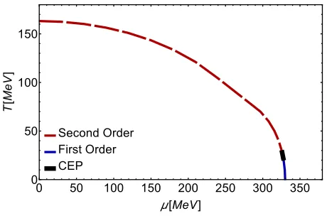
Figure 2.QCD phase diagram obtained from the solutions to the equations that determine the coupling constants. This are computed withTc
0(µq =0)=165 MeV andµcq(T =0) =330 MeV. The second order transitions are indicated by red line and the first order transitions by the blue line. These areas represent the results directly obtained from our analysis.
At point (A), the phase transition is second order, hence the square of the pion thermal mass, evaluated atv=0 andT =Tc0, is given by
m2
Second Order
First Order
CEP
0 50 100 150 200 250 300 350
0 50 100 150
μ[MeV]
T
[
M
eV
]
Figure 1.QCD phase diagram obtained from the solutions to the equations that determine the coupling constants. This are computed withTc
0(µq =0)=170 MeV andµcq(T =0) =340 MeV. The second order transitions are indicated by red line and the first order transitions by the blue line. These areas represent the results directly obtained from our analysis.
Second Order
First Order
CEP
0 50 100 150 200 250 300 350
0 50 100 150
μ[MeV]
T
[
M
eV
]
Figure 2.QCD phase diagram obtained from the solutions to the equations that determine the coupling constants. This are computed withTc
0(µq =0)=165 MeV andµcq(T =0) =330 MeV. The second order transitions are indicated by red line and the first order transitions by the blue line. These areas represent the results directly obtained from our analysis.
At point (A), the phase transition is second order, hence the square of the pion thermal mass, evaluated atv=0 andT =Tc0, is given by
m2
π(0,T0c, µq=0)=−a2+ Π(T0c, µq=0)=0. (31) At point (B), the phase transition is first order (degenerates minimal), therefore the minimum we are considering is the one with a vacuum expectation value different from zero, which we callv1. This last condition can be written as
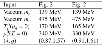
Table 1.Physical inputs from points A and B and for vaccum bosons masses
Input Fig. 2 Fig. 2 Vaccummπ 139 MeV 139 MeV
Vaccummσ 475 MeV 475 MeV
T0
c(µq=0) 170 MeV 165 MeV
µ0c(T =0) 340 MeV 330 MeV (λ, g) (0.87,1.57) (0.91,1.61)
m2
π(v1,0, µcq)=λv1−a2+ Π(0, µcq)=0, (32) In Eq. (32), we notice that a new unknown appears: v1, that is, the value of the non-vanishing minimum. In order to guarantee that the order of the transition in points A and B is consistent with the physical input, we need to add counter-termsδa2andδλto the bare constantsa2andλ, respectively,
in the tree level potential
Vtree=−a2 2v2+
λ
4v4
→ −(a2+2δa2)v2+(λ+δλ)
4 v4. (33)
Therefore the set of conditions necessary to determinev1and the counter-terms is
∂2Veff
∂v2 (v=0,T =Tc, µq=0)=0, (34)
∂Veff
∂v (v=0,T =0, µq=µ
c q)=0,
∂Veff
∂v (v=v1,T =0, µq=µ
c q)=0,
Veff(v=0,T =0, µ
q=µcq)=Veff(v=v1,T =0, µq=µcq). (35)
The expressions in Eq. (34) indicate that the effective potential is second order whenµ =0 and T =Tcand the three expressions in Eq. (35) indicate that the effective potential has two degenerated minima at the phase transition and thus that the transition is first order whenT =0 andµq=µcq. The above set of conditions, Eqs. (31), (32) and (35), represent the five algebraic equations that determine the values ofλandg. Finally, we can explore the QCD phase diagram.
5 Results
6 Summary
In this work we have used the linear sigma model with quarks to explore the QCD phase diagram from the point of view of chiral symmetry restoration. We have computed the finite temperature effective
potential up to the contribution of the ring diagrams to account for the plasma screening effects. For
high quark chemical potential we introduced a boson chemical potentials linked to the high baryon abundanceand.
Our approach was to determine the model’s couplings using physical inputs such as the vacuum pion and sigma masses, the LQCD value for the critical temperature atµq =0 and the conjectured end point value ofµB of the transition line atT =0. The set of conditions that determine the cou-plings enforce the requirement that at high temperature the transition is second order whereas at low temperature is first order.
In order to provide a more robust CEP’s location, we need to include the temperature and density modifications to the couplings which has been shown useful to describe the inverse magnetic catalysis phenomenon [8]. For more explicit details, the reader us referred to Ref [9].
Acknowledgments
Support for this work has been received in part by UNAM-DGAPA-PAPIIT grant number IN101515 and by Consejo Nacional de Ciencia y Tecnología grant number 256494.
References
[1] A. Ayala, J. D. Castaño-Yepes, J. J. Cobos-Martínez, S. Hernández-Ortiz, A. J. Mizher, A. Raya, Int. J. Mod. Phys. A31, 1650199 (2016).
[2] A. Ayala, A. Bashir, J.J. Cobos-Martínez, S. Hernández-Ortiz, A. Raya, Nucl. Phys. B897, 77-86 (2015).
[3] M. Le Bellac,Thermal Field Theory(Cambridge Monographs on Mathematical Physics), Cam-bridge University Press, 1996.
[4] L. Dolan and R. Jackiw, Phys. Rev. D9, 3320-3341 (1974). [5] C. O. Dib, O. R. Espinosa, Nucl. Phys. B612, 492-518 (2001). [6] T. Bhattacharyaet al., Phys. Rev. Lett.113, 082001 (2014).
[7] R. Hagedorn, Nuovo Cim. Suppl.3 (1965) 147; Nuovo Cim. A56 (1968) 1027; See also K, Fukushima, T. Hatsuda, Rept. Prog. Phys.74, 014001 (2011).
[8] A. Ayala, L. A. Hernández, M. Loewe, A. Raya, J. C. Rojas, R. Zamora, Phys. Rev. D 96, 034007 (2017); A. Ayala, C. A. Dominguez, L. A. Hernández, M. Loewe, A. Raya, J. C. Rojas, C. Villavicencio, Phys. Rev. D94, 054019 (2016); A. Ayala, M. Loewe, R. Zamora, Phys. Rev. D91, 016002 (2015); A. Ayala, M. Loewe, A. J. Mizher, R. Zamora, Phys. Rev. D90, 036001 (2014).