Representation and self-adaption in genetic algorithms

VICTORIA

~

UNIVERSITY

•

:

n

z z 0 .

0

.

:

DEPARTMENT OF COMPUTER AND

MATHEMATICAL SCIENCES

Representation and Self-adaption in

Genetic Algorithms

Robert Hinterding

(69 COMP 23)

February, 1996

(AMS

:

68T05)

TECHNICAL REPORT

VICTORIA UNIVERSITY OF TECHNOLOGY

DEPARTMENT OF COMPUTER AND MATHEMATICAL SCIENCES

P

0

BOX 14428

MCMC

MELBOURNE, VICTORIA 8001

AUSTRALIA

DEPARTMENT OF COMPUTER AND

MATHEMATICAL SCIENCES

Representation and Self-adaption in Genetic Algorithms

1

Robert Hinterding

email: [email protected]

TECHNICAL REPORT

69COMP23

December 1995

Department of Computer and Mathematical Sciences

VICTORIA

UNIVERSITY OF TECHNOLOGY

PO Box 14428 MMC, Melbourne 3000, Australia

Telephone +61 3 9688 4249

Facsimile +61 3 9688 4050

1 _{A version of this report was presented at the Korea-Australia Joint Workshop on}

Abstract

Representation and reproduction operators are important issues in Ge-netic Algorithms(GAs). When optimising numerical functions some re -searchers advocate using floating point representation instead of bit-string representation. Floating point representation is also used in Evolutionary Strategies(ESs) and Evolutionary Programming(EP). We show that it is not the representation that is responsible for the improved performance,

but the mutation operator. By using Gaussian mutation with bit-string representation we improve the performance of GAs. We then introduce self-adaption which raises the performance to that of ESs. We also show that keeping bit-string representation can have advantages to the efficiency of GAs.

1

Introduction

In

Genetic Algorithms ( GAs ), bit-flip mutation is unchallenged when bit-string representation is used. Most research has concentrated on other issues as mu-tation is generally considered to be a background operator used only to replace bits lost by crossover (Holland, 1992; Goldberg, 1989). Other forms of muta-tion have been used when bit-string representamuta-tion was inappropriate or was not used. Examples of GAs not using bit-flip mutation are Order based GAs (Davis, 1991), Grouping GAs (Falkenauer & Delchambre, 1992) and real valued GAs (Wright, 1991).

The other areas of Evolutionary Computation, Evolutionary Programming · (EP) and Evolutionary Strategies (ES) consider mutation to be far more

impor-tant (Back

&

Schwefel, 1993). In fact in EP, mutation is the only reproduction operator.

In Hinterding, Gielewski

&

Peachey (1995) it was shown that by considering function variables as genes in GAs using bit-string representation, important characteristics about representation and mutation could be discerned. By con-sidering mutation as an independent reproduction operator, its importance to GAs was demonstrated. The probability distributions of bit-flip mutation on genes using Gray or binary decoding were developed and showed that neither of these types of mutation is ideal as the changes to the function variables cluster very strongly about zero and are sensitive to the granularity used to represent the function variables.

When we consider the function variables to be the genes, we can develop other mutation operators besides bit-flipping. We now have a much larger al-phabet for the genes, and can consider mutation to generate a normal distribu-tion of changes. This can be simulated by adding Gaussian noise to gene values (Gaussian mutation). Gaussian mutation is not new to Evolutionary Compu-tation as it has been used in both Evolutionary Strategies and Evolutionary Programming (Back

&

Schwefel, 1993; Saravanan & Fogel, 1994).

We investigate the usefulness of Gaussian mutation in GAs used for nu-meric function optimisation. We maintain bit string representation so that the distinction between genotype and phenotype is maintained, and control over \ the granularity of representation is possible. Hence, the changes to the GA

Self-adaption is a powerful tool that has long been used in ESs (Back, 1992; Schwefel, 1995) to set the values of the strategy parameters. Back (1992) used self-adaption in GAs to control the probability for flipping bits representing one of more function variables. We use self-adaption to allow the GA to control the variance for Gaussian mutation.

We show that Gaussian mutation can give superior results to bit-flipping mutation for most functions, in particular Gaussian mutation is better for some of the "deceptive" problems. We also show that using self adaption to control the variance for Gaussian mutation gives significant improvement for most of the functions and that the changes of the variance over time are appropriate for the different types of functions being optimised.

In ES and EP, the function variables are represented as floating point num-bers. In GAs the "traditional" representation is bit-strings that are mapped to fixed-point reals, although a number of researchers advocate using floating point numbers (Davis, 1991; Michalewicz, 1994; Wright, 1991). We investi-gate whether bit-string repesentation has any advantages over floating point representation.

2

Gaussian mutation

By considering the variables of the function that are being optimised as the genes, we can define new mutation operations besides the standard bit-flipping mutation operator. The distribution of changes to genes by using bit-flipping mutation with either Gray or binary decoding is not ideal. When Gray decoding is used, most of the changes are very small and it is very sensitive to choosing the correct granularity. Binary decoding has the effect that all possible changes are equally likely, but there are large gaps in the distribution of possible changes. It seems reasonable therefore that mutation which has normally distributed changes could produce better results and reduce the sensitivity to choosing the length of the variables.

We implement fixed Gaussian mutation by first decoding the gene to an unsigned integer and then adding Gaussian noise, the new value is then encoded and replaces the gene in the chromosome. Gaussian noise is obtained from a normally distributed random variable which has a mean of 0 and a standard deviation of 0.1 times the maximum value of the gene. The value 0.1 was chosen so that an interval of more than 3 standard deviations each side of the mid-point of the range will encompass most of the range. With this scheme new gene values can exceed the range at either end of the range if the original gene value is sufficiently far away from the mid-point of the range. These values can be treated in two ways, we can either truncate the value back to the end-point it exceeded, or the value can be allowed to "wrap around", that is multiples of the range are added or subtracted to give a value within the range.

2.1

Self-adaptive Gaussian Mutation.

In ESs and in meta-EPs self-adaption is used to control strategy parameters. Here learning is used to adjust the strategy parameters while searching for the optimum. One of the problems with Evolutionary Computation algorithms is finding values for the parameters which will optimise their performance. The optimal values for the parameters are generally not constant during the whole run, and also depend on the function to be solved. Hence allowing the algorithm to adjust the values during the run can have large benefits.

We add one value to each chromosome, which will control the standard deviation of the Gaussian mutation used on the genes in the chromosome that will be mutated. This value is allowed to participate in crossover and mutation, but does not contribute directly to the fitness of the solution. This simple scheme should allow us to test its utility.

We implement self-adaptive mutation by adding an extra gene to the front of all chromosomes. The values of this gene are allowed to vary from 0.00002 to 0.2. This gene is allowed to participate normally in crossover, but when the chromosome is to be mutated the following steps are followed:

1. decode the gene to a value.

2. apply Gaussian noise to the value using a standard deviation of 0.013. This value was found experimentally to give good results.

3. use this value as the standard deviation of the Gaussian noise to mutate the other genes in the chromosome.

4. write the mutated special gene and the mutated genes back to the chro-mosome.

When the initial population is created, the special genes are given random values around 0 .1.

3

Numeric GA Test functions

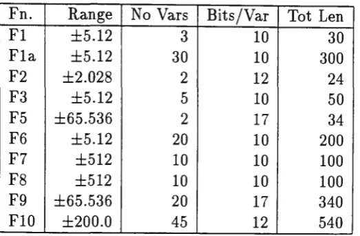
The test functions have been taken from a number of sources, and more difficult functions have been included. Fl - F5 are from De Jong (1975), F6 - F8 are from Scott

&

Whitley (1993), F9 is from Hoffmeister and Back (1992), and FlO is from Michalewicz (1994). The range, number of variables and number of bits used to represent each variable is summarised in Table 1.

• Fl Sphere Model. This is a continuous, strictly convex, unimodal func-tion. The solution is at

x*

=

(0, ... , Of;

fi(x*)

=

0. This is a scalable problem, with n

=

3 the problem is easy, Hoffmeister

&

Back (1992) use

n = 30, which we call test function Fla.

• F2 Rosenbrock's Function. This is a continuous, unimodal, bi-quadratic function of two variables. It is a standard test function in optimisa-tion which was proposed by Rosenbrock (1960). The soluoptimisa-tion is at

x*

=

• F3 De Jong Step Function. This is a simple linear but discontinuous func-tion, which consists of many small plateaus. Due to this characteristic f3 has a lot oflocal optima. The solution is at Xi E [-5.12, ... , -5); h(x*) =

0.

• F5, Shekel's Foxholes. This is a continuous, non-linear, multimodal func-tion proposed by Shekel ( 1971). It is a difficult problem as it consists of a large plateau with some holes in it which have different objective values at their bottoms, while the plateau is made up of equal objective values. The solution is at xi

=

(-32, -32f; fs(x*) ~ 1.

• f6, Generalised Rastrigin's Function. This function is a scalable, contin-uous, mulitmodal test function which is made from Fl by modulating it with Acos(27rxi)· It was first proposed by Rastigin as a 2-dimensional problem (Torn

&

Zilinskas, 1989), and has been generalised by Rudolph (1991) as a test function for distributed parallel ESs. The solution is at x*

=

(0, ... , Of; fB(x*)

=

0.

• F7, Schwefel's Fu·nction. This is a multimodal function characterised by a second-best minimum which is far away from the global optimum. The solution is at x* = (421, ... ,421f; h(x*) = 0.

• F8, Griewangk's Function. This function is difficult for GAs because the variables are strongly independent. The solution is at x* = (0, ... , o)T; fs(x*) = 0.

• F9, Schwefel's Problem 1.2. This is a continuous, unimodal function which comes from the set of test functions that Schwefel (1977) once used to compare the performance of several optimisation methods. The difficulty of this function results from the fact that searching along the coordinate axes only gives a poor rate of convergence. The solution is at x* =

(0, ...

'of; fg(x*)

=

0.

• FlO, Michalewicz's dynamic control problem. The range of x is (-200, 200), the function has a minimum at 16,180.4.

4

The GA

The Genetic Algorithm used is a steady-state GA based on the description of OOGA in Davis (1991). Tournament selection is used with a tournament size of 2 as this was faster and gave comparable results to roulette wheel selection with linear normalisation. It was developed using Smalltalk/V for Windows. The following parameters can be set:

• Population Size - set the size of the population.

Fn. Range No Vars Bits/Var Tot Len Fl ±5.12 3 10 30 Fla. ±5.12 30 10 300 F2 ±2.028 2 12 24 F3 ±5.12 5 10 50 F5 ±65.536 2 17 34 F6 ±5.12 20 10 200 F7 ±512 10 10 100 F8 ±512 10 10 100 F9 ±65.536 20 17 340 FlO ±200.0 45 12 540

Table 1: Function Characteristics

reproduction are discarded while they still count as an evaluation. We determine whether two chromosomes are the same by comparing their genotypes.

• Number of Evaluations - set the number of evaluations for the run. We use evaluations rather than generations so that we can comp&re between runs where the population size and replacement rate are different.

• Replacement Rate - set the percentage of the population that will be replaced by reproduction in one generation. The rate can be set from 0 to 1003.

• Crossover Rate - set the percentage of the replacement population that will be replaced by crossover in one generation. The remainder of the replacement population will be produced by mutation. The rate can be set from 0 to 1003.

• Poisson Mutation - use a Poisson distributed random variable to deter-mine how many genes to mutate in a chromosome. If this is false only one gene per chromosome is mutated.

• Poisson Mean - set the mean ( >.) for the Poisson distributed random variable. This controls the number of genes that will be mutated in the chromosome if Poisson Mutation is true.

Two point crossover was used for all the experiments, although others were available.

fixed self-adaptive

Fn. Best

A

Crx. Rep Best

A

Crx. Rep

Fl 3570# 1.5 50 80 3830# 2 40 60

Fla 4.6e-2 1.5 50 20 9e-5 10 40 60 F2 8.9e-5 5 I 40 90 7490# 5 10 80

F3 1895# 2 ' 30 30 2550# 1 50 50

I

F5 2690# 2 50 80 3830# 1 60 60

F6 1.9e0 1.2 50 40 3.leO 1. 7 60 60

F7 5.6el 2.5 50 20 7.3el 4 60 90

F8 l.6e-l 1 60 20 7.9e-2 1.5 40 20 F9 3.6e2 2 10 90 1.4e2 10 10 40 FlO 4.2e4 2.5 30 90 2.6e4 15 10 20

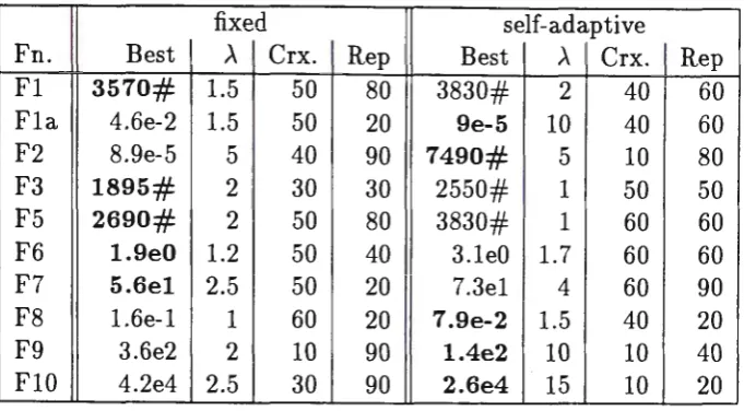
Table 2: Results for Gaussian mutation

the mix of these operators that produces the best results within a given number of evaluations.

The mutation rate for the GA is (100% - Crossover rate). The mutation rate is the percentage of chromosomes of the replacement population that will undergo mutation. If Poisson Mutation is false, then mutation of one gene is carried out. If Poisson Mutation is true, then the number of genes to be mutated in a chromosome is determined by sampling a Poisson distributed random variable with mean A. If n genes are to be mutated in a chromosome, then we repeat n times: select a random gene from the chromosome and mutate the gene. Note that mutation is now controlled by the crossover rate, the number of genes in the chromosome to mutate, and the standard deviation of the Gaussian noise if Gaussian mutation is used.

5

The Experiments

5.1

Gaussian Mutation

Table 2 show the results for the GAs using fixed and self-adaptive Gaussian mutation. Three sets of runs were performed on each problem, so that the parameters could be varied to get some indication of the best settings for each problem. The parameters that were varied were the crossover (and mutation rate), the replacement rate, and whether Poisson based mutation used. In the set of runs where Poisson based mutation was used, the Poisson mean was varied. In each run the GA is run on the problem 20 times and the results are averaged.

Fn. Evals Best

A

µ Crx. Rep Fl 4,000 2510# 2.7 0.09 40 20 Fla 12,000 7.9e-2 2.1 0.007 50 40 F2 12,000 3.3e-5 3.6 0.15 20 80 F3 6,000 5090# 3 0.06 10 70 F5 4,000 1650# 2.4 0.07 10 90 F6 12,000 2.8el 2.2 0.011 80 90 F7 12,000 2.5e2 4.2 0.042 10 40 F8 12,000 l.2e-l 3 0.03 40 40 F9 12,000 9.5e2 5.8 0.017 10 90 FlO 20,000 9.6e4 3.4 0.006 10 20

Table 3: Results from bit-flip mutation

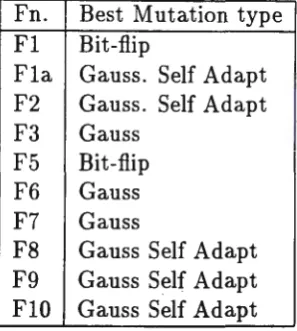
Fn. Best Mutation type Fl Bit-flip

Fla Gauss. Self Adapt F2 Gauss. Self Adapt F3 Gauss

F5 Bit-flip F6 Gauss F7 Gauss

F8 Gauss Self Adapt F9 Gauss Self Adapt FlO Gauss Self Adapt

Table 4: Best results by GA type

the crossover rate for the best results, and "rep" show the replacement rate which gave best results for a crossover rate of 503.

The figures in bold show the best results obtained for that function in the table.

In Tables 2 and 3, "A" shows the Poisson mean which gave the best results. The data from Table 3 is from Hinterding, Gielewski and Peachey (1995), the same same GA was used to produce these results. Here bit-flip mutation and Gray encoding was used.

5.2

Gene Length

30

fixed ~

25 self adapt

-8-20

% ₁₅

succ.

10

5

0

0 3000 6000 9000 12000

Evals

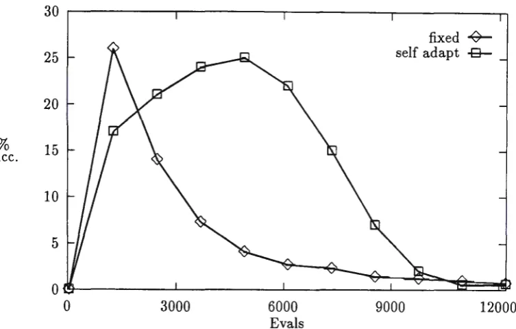
Figure 1: Percentage successful mutations for Fla

In Evolutionary Algorithms where floating point representation is used, the search space is huge as floating point representation gives a very fine granularity. Experiments were run on all the functions and the number of bits used to represent genes was varied from 10 to 30 bits. These runs used fixed Gaussian mutation.

From the results in Table 5, ·we see that for some of the functions the

gene length has no significant effect while for others the shorter gene length gives better results. These differences could be explained by the change in

granularity or by changes to the efficiency of crossover. If the optimum can be

found during the run, having a coarser granularity makes the optimum easier to find. Where the optimum is not likely to be found during the run (on the more difficult problems), the granularity used may have only a small effect. Crossover could be effected by finer granularity (and longer representation) as

a greater percentage of crossovers will produce only a very small change in the

function value. The results are generally worse for longer gene representation, but do not deteriorate as quickly as when bit-flip mutation is used (Hinterding

et al. , 1995).

5.3

Recombination or

Crossover

In GAs using bit-string representation crossover points can occur anywhere

Fn. 10 bits 14 bits 18 bits 22 bits 26 bits 30 bits

Fl 2690# 4010# l.6e-8 l.6e-8 4.le- 7 9.9e-7

fla 4.6e-2 5.0e-2 4.8e-2 4.9e-2 4.5e-2 4.5e-2 F2 3.0e-5 2.4e-4 2.3e-4 2.le-4 1. 7e-4 3.3e-4

F3 1895# 3740# 3125# 2510# 3740# 2510#

F5 2690# 3130# 2690# 3130# 4010# 4010#

F6 l.7e0 l.9e0 2.4e0 2.2e0 l.9e0 2.leO

F7 3.7e2 4.le2 4.le2 4.3e2 5.4e2 6.2e2

F8 2.8e-l 2.8e-l 3.0e-1 3.5e-l 8.3e-l 8.4e-l

F9 l.3e3 l.8e3 l.7e3 2.3e3 2.5e3 2.8e3

FlO l.le5 l.4e5 l.7e5 l.8e5 2.le5 2.4e5

Table 5: Results for Varying Gene Length

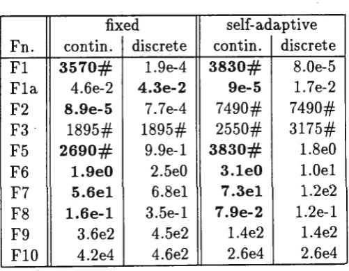
fixed self-adaptive

Fn. con tin. discrete contin. discrete Fl 3570# l.9e-4 3830# 8.0e-5

Fla 4.6e-2 4.3e-2 9e-5 1. 7e-2

F2 8.9e-5 7.7e-4 7490# 7490#

F3 · 1895# 1895# 2550# 3175#

F5 2690# 9.9e-l 3830# l.8e0

F6 1.9e0 2.5e0 3.leO l.Oel

F7 5.6el 6.8el 7.3el l.2e2

F8 1.6e-1 3.5e-l 7.9e-2 l.2e-l

F9 3.6e2 4.5e2 l.4e2 l.4e2

FlO 4.2e4 4.6e2 2.6e4 2.6e4

0.12

Fla

4-0.1 F7

-e-F6 ~

0.08

Std.

0.06

Dev.

0.04

0.02

0

0 3000 6000 9000 12000

Evals

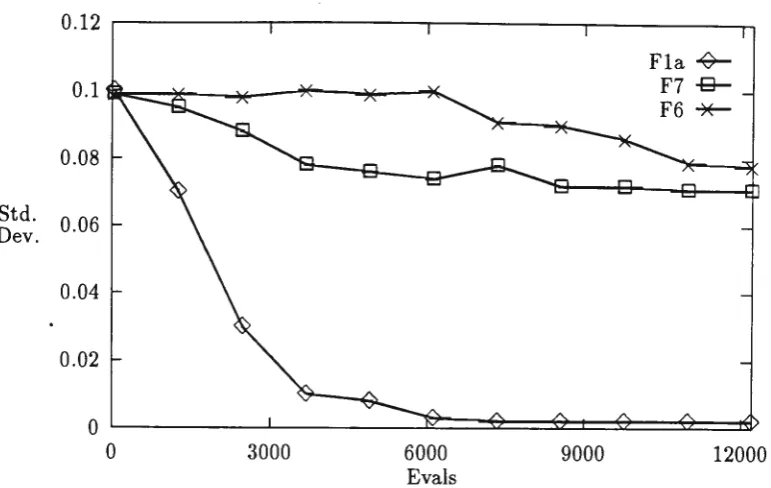
Figure 2: Change in variance in Self Adaptive GA

where crossover points can occur within the genes ( contin.) and the GA where crossover points can only occur between genes (discrete). While this is only a simple experiment as other forms of recombination are also used, the results indicate that crossover is beneficial.

6

Discussion and Conclusions

By treating the function objective variables as genes, we are able to introduce new mutation operators which could not be envisioned when we treat the binary bits of the chromosome as genes.

We can see from Table 4 that GAs using Gaussian mutation produced the best results for most of the functions. We can therefore conclude Gaussian mutation is a useful mutation operator and is in most cases superior to bit flip mutation. Our GAs use mutation as an independent reproduction operator, that is a new individual (chromosome) is produced by either crossover or mu-tation and not both. By comparing Tables 2 and 3 we can see that when using Gaussian mutation, the crossover rate is more often near 503. We speculate that this could be due to Gaussian mutation producing values that crossover can more easily utilise.

1000

100

-500

x(l)

Figure 3: Schwefel's Function

Gaussian mutation during the run.

500

Figure 2 shows the change in the variance of the Gaussian mutation when self-adaption is used. For Fla the variance is decreased as expected and is very small towards the end of the run, while the variances for F6 and F7 are both kept high throughout the run. Function F6, Rastrigins's function is characterised by many local optima, in this case keeping the variance high would optimise the chance of hitting a peak. F7 is a "deceptive" problem with a local optimum a

long way from the optimum, again keeping the variance high is advantageous.

This shows that self adaption is capable of adapting to different situations successfully.

Part of the improvement for function F7, with the GAs using Gaussian mutation we attribute to the fact that "wrap around" is used in the Gaussian mutation operator. F7 is like the "deceptive" problems (Deb

&

Goldberg, 1992) in that it has a second best optimum near one end of the range while the optimum is at the other end (see Fig 3). By allowing values being mutated to "wrap around" a much short path to the optimum value is provided. This result looks very promising and could eliminate a class of "deceptive" problems. When we now compare our results with those of ESs in Hoffmeister and Back (1992) (see Table 7), we see that our GAs using Gaussian or self-adaptive Gaussian mutation now have comparable performance. ESs appear to do bet-ter on the "smoother" functions, while our GAs do betbet-ter on the "rougher" functions.

improve-Fn. ES Our GAs

Fla le-5 9e-5

F2 5000# 7490#

F3 leO 1895#

F5 3.5e0 2690#

F6 6e0 1.9e0

F9 2el 1.4e2

Table 7: Comparison of results with Hoffmeister and Back

ment reported by switching from bit-string to floating point representation in GAs(Davis, 1991; Wright, 1991) is due the different mutation operators used rather than any change in representation.

Acknowledgments

The author would would like to thank Ted Alwast, Tom Peachey and Harry Gielewski for their help and useful comments.

References

Back, T. 1992. Self-adaption in Genetic Algorithms. In: Proceedings of the First European Conference on Artificial Life. Cambridge: MIT Press. pp. 263-271.

Back, T., & Schwefel, H-P. 1993. An Overview of Evolutionary Algorithms. In: Evolutionary Computation. l, vol. 1. MIT Press.

Davis, L. ( ed). 1991. Handbook of Genetic Algorithms. Van Nostrand Reinhold.

De Jong, K. A. 1975. An analysis of the behaviour of a class ofgenetic adaptive system. Doctoral dissertation, University of Michigan.

Deb, K., & Goldberg, D. E. 1992. Analysing Deception in Trap Functions.

Jn: Whitley, L. D. ( ed), Foundations of Genetic Algorithms - 2. Morgan Kaufmann.

Falkenauer, E. A.,

&

Delchambre, A. 1992. A Genetic Algorithm for Bin Packing and Line Balancing. In: Proceedings of 1992 IEEE International Confer-ence on Robotics and Automation(RA92}. pp. 1186-1193.

Goldberg, David E. 1989. Genetic Algorithms in Search, Optimization f3 Ma-chine Learning. Addison-Wesley.

Fifth International Conference on Genetic Algorithms. Urbana-Champain: Morgan-Kaufmann. pp 177-183.

Hinterding, R., Gielewski, H., & Peachey, T. C. 1995. The Nature of Mutation

in Genetic Algorithms. In: Eshelman, L.

J.

(ed), Proceedings of the Sixth

International Conference on Genetic Algorithms. Morgan Kaufmann. pp.

65-72.

Hoffmeister, F.,

&

Back, T. 1992 (Feb). Genetic Algorithms and Evolution

Strategies: Similarities and Differences. Technical Report No. SYS-1/92.

Systems Analysis Research Group, University of Dortmund, Germany.

Holland,

J.

H. 1992. Adaption in Natural and Artificial Systems. 2nd edn. MIT

Press.

Michalewicz, Z. 1994. Genetic Algorithms

+

Data Structures

=

Evolution

Pro-grams. 2nd edn. Springer - Verlag.

Rosenbrock, H. H. 1960. An automatic method for finding the greatest or least

value of a function. In: The Computer Journal. 3, vol. 3. pp 175-184.

Rudolph, G. 1991. Global Optimization by means of distributed evolution

strategies. In: In Parallel Problem Solving from Nature. Lecture Notes in

Computer Science, vol. 496. Springer-Verlag.

Saravanan, N ., & Fogel, D.B. 1994. Learning Strategy Parameters in

Evolu-tionary Programming: An Empirical Study. In: Sebald, A.V.,

&

Fogel,

L.J. (eds), Proceedings of the Third Annual Conference on Evolutionary

Programming. World Sci.

Schwefel, H-P. 1977. Numerische Optimierung von Computer-Modellen mittels

der Evolutionsstrategie. Interdisciplinary systems research, vol. 26. Basel:

Birhauser.

Schwefel, H-P. 1995. Evolution and Optimum Seeking. Sixth-Generation

Com-puter Technology Series. Wiley.

Shekel, J. 1971. Test functions for multimodal search techniques. In: Fifth

Annual Princeton Conference on Information Science and Systems.

Torn, A., & Zilinskas, A. 1989. Global Optimization. Lecture Notes in Computer

Science, vol. 350. Springer-Verlag.

Wright, A.H. 1991. Genetic Algorithms for Real Parameter Optimization. In:

Rawlins, G.E. ( ed), Foundations of Genetic Algorithms. 3, vol. 3. Morgan