DYNAMIC SPECTRUM ACCESS IN WIRELESS NETWORKS

DYNAMIC SPECTRUM ACCESS IN WIRELESS

NETWORKS

1

T. N. Vaishnavi,

Dr. T. K. Shanthi,

1

P.G Student,

Associate Professor,Department of ECE,

Thanthai Periyar Government Institute of Technology, Vellore-2, Tamilnadu, India

ABSTRACT

The primary design objective for an efficient secondary user access strategy is to be able to measure spatiotemporally fragmented bandwidth while limiting the amount of interference caused to the primary users. In this paper, a secondary user access strategy is proposed which is based on measurement and modelling of the whitespace as perceived by the secondary users in a WLAN. A secondary user monitors and models its surrounding whitespace, and then accesses the available spectrum so that the effective secondary throughput is maximized while the resulting interference to the primary users is limited to a pre-defined bound.

First, analytical expressions for the secondary throughput and primary interference have been developed, and then JiST based simulation experiments has been performed to validate the effectiveness of the proposed access strategy, and its performance has been evaluated numerically using the developed expressions. The results show that the proposed access strategy is able to consistently sense between 90% and 96% of the available whitespace bandwidth, while keeping the primary users disruption less than 5%.

Key Words: Dynamic Spectrum Access, Secondary User Access Strategy, Whitespace Modelling

I INTRODUCTION

1.1

Spectrum Allotment

Recent research on Dynamic Spectrum Access (DSA) has paved the way for a set of Secondary Users (SU) to access underutilized spectrum between Primary Users’ (PU) transmissions in space, time and frequency. It has been shown

based on their respective traffic priorities. For example, consider a VoIP primary user network utilizing a 2.4 GHz band. Along with the high-priority primary user devices there are coexisting low priority secondary user devices (e.g. sensors, laptops etc.) using the same band.

1.2

Objective

The objective here is to design a strategy to allow the secondary users to access the channel and utilize the bandwidth without disrupting or restricting the high-priority primary user devices. Coexistence between these systems can be achieved through spatial or frequency separation. We propose in this paper, an optimal secondary user access strategy to utilize temporal separation between primary and secondary devices accessing the same radio frequency (RF) spectral segments within a WLAN.

II SPECTRUM ANALYSIS

2.1

Challenges

The secondary users’ goal is to access the idle times between the transmissions of primary users. These idle times or

whitespaces typically last for short durations (i.e. order of milliseconds) in between the active data transmissions of PUs. The primary challenge in designing an access strategy for the SUs is how to minimize the disruption to the primary users while maximizing the secondary user throughput without deterministic knowledge about the future occurrences of whitespaces and their durations. A number of research groups have started addressing the related issues 6and this project proposes a new optimal solution to this problem.

2.2

Arithmetic Bandwidth Distribution

2.3

Contributions

The contributions of this project are as follows. First, we present the whitespace characteristics created by different primary user traffic scenarios. Note that the PU traffic scenarios represent a significant extension over the simplistic topologies considered in the 802.11 based DSA. Second, we develop a stochastic model of the whitespace for identifying effective transmission opportunities for the SUs. Third, based on this model, a comprehensive channel access strategy is developed to facilitate bandwidth scavenging by the SUs. Finally, we experimentally demonstrate that the proposed access strategy is able to accomplish the targeted goals of high SU throughput and low disruption to PUs for multiple traffic characteristics and in the presence of multiple SUs.

Prioritized device coexistence within CSMA based WLANs can be achieved by using different inter frame spacing (IFS) periods for different user and/or traffic classes. MAC protocol 802.11e, for instance, uses different Arbitration IFS (AIFS) periods to provide CSMA based prioritized access among different device and/or traffic classes. When a channel is found free, a node waits for a specific AIFS periods depending on the device or traffic class, before it attempts to send a packet. For higher priority primary traffic, a node waits for a smaller AIFS period. This ensures when multiple nodes contends for the channel, the primary users’ nodes (with smallest AIFS) wins. While providing

reasonable access differentiation, these approaches rely only on the instantaneous channel status (i.e. free or busy) for granting access. This leads to undesirable disruptions to the PU traffic as follows. Consider a situation in which an SU intends to transmit a packet and it does so after finding the channel free (i.e. a whitespace) for the AIFS specified for the SUs. Now, in the middle of this SU’s packet transmission if a PU in the vicinity intends to send a

packet, it needs to wait until the current SU transmission is over. This causes an undesirable delay for the PU traffic, which in turn will affect the PUs’ application performance. Since this is mainly a result of the SUs’ reliance only on

the instantaneous channel state, a more robust approach for the SUs would be to also consider the long term whitespace model. The following DSA approaches attempt to accomplish that. Networks with primary users running 802.11 MAC protocol have recently been investigated for possible dynamic spectrum access by secondary users. The authors developed a methodology for formally analyzing the whitespace available within 802.11 primary traffic in infrastructure mode. The key idea is to model the whitespace as a semi-Markov process that relies on the underlying 802.11 state model involving DIFS, SIFS, DATA, and ACK transactions. The model describes the whitespace profile in terms of holding times of the idle and busy states of the channel. Building on this whitespace model, the authors further develop a WLAN dynamic spectrum access strategy for secondary users in which the SUs utilize packet size slots for the channel access. At the beginning of each slot, an SU senses the channel and if the channel is free then it transmits with a specified probability that is calculated from previous measurement. The objective is to minimize PU disruption and maximize SU throughput.

The use of time-slotting in their approach requires time synchronization across the secondary users. In the proposed access mechanism in this paper, the need for such inter-SU time synchronization is avoided via asynchronous whitespace access based on a stochastic whitespace modelling approach.

protocol (e.g. CSMA) within those identified whitespace portions in order to minimize the inter-SU access contentions. This makes multiple SU support a natural extension in our proposed approach.

Fig : 2.1 Primary user topologies and the traffic flows

The PUs in this framework cooperates with the SUs through pricing strategies and subscription fees to facilitate spectrum sharing. These approaches require the PUs to have knowledge of the SUs presence. In contrast, the proposed mechanism in this paper, no such cooperation is assumed, thus no changes in the PUs behavior is needed. The idea here is to develop an access mechanism for the SUs for scavenging the PUs’ leftover bandwidth, without the PUs being aware of such scavenging. For example, data-enabled hand-held devices should be able to scavenge bandwidth in a WLAN without the primary VoIP handsets being aware of the scavenging process.

As for the primary traffic profile, the researchers model the primary users’ packet arrival intervals and packet durations as two separate Poisson processes. Similarly, it uses an ONOFF pattern, where the durations of the idle and busy states follow two exponential distributions. A Markov chain with known transition probabilities is used for modelling primary user behavior. In line with these work, the proposed mechanism in this work is evaluated for a large variety of PU traffic profiles under single and multiple SU scenarios.

III BANDWIDTH MEASUREMENT

3.1

Analysis

Figure 3.1 : Impacts of PU topology with Uniform, Poisson, TCP and Video Stream traffic on whitespace distributions. The graphs (a), (b), (d), and (e) show the pdf, along with (c) and (f) presenting the

corresponding cumulative distribution function (cdf) from 0 to 1 ms.

3.2

Whitespace Measurement and Model

A secondary user measures the available whitespace by detecting the received signal strength (RSSI) at a given channel frequency. The RSSI threshold used in this paper to determine whitespaces is the corresponding RSSI value (-108 dBm) of the Carrier Sense (CS) range defined by the 802.11 protocol. Such whitespaces are a function of the physical locations, topology, traffic profile, and routing protocols used by the primary users. An SU detects the channel whitespace through periodic channel sensing with a sensing period Tp. Based on these sensed samples, the whitespace is modeled using its probability density function, w(n), which represents the probability that the duration of an arbitrarily chosen whitespace is nTp. The quantity w(n) is periodically computed in order to capture any dynamic changes in the primary user behavior.

3.3.

Diverse Primary User Topology and Traffic Profile

In order to represent varying 802.11 Ad-hoc network topologies and traffic characteristics, the following three scenarios are established (see Fig. 3.1): (TOP1) a linear chain topology with a single multi-hop primary flow, (TOP2) two multi-hop flows in a network on two intersecting linear chains, and (TOP3) two multihop flows in a parallel chain network. In each case, the secondary users are within the CS range of all primary users. Note that these multi-hop scenarios represent significant extensions over the simplistic topologies considered in the 802.11 based DSA.

The traffic profile and data rate of the primary user can directly affect the total amount and statistical properties of the available whitespace as viewed by the secondary users. We model three types of PU traffic, namely, bidirectional UDP with a fixed packet size, TCP, and a Video Stream. For the UDP traffic, the packet arrival intervals are modelled as:

2) A Poisson process with mean packet arrival interval of δ ms. The packet arrival intervals for each Uniform and Poisson flow is varied from low to high values to represent varying intensity of primary traffic.

3.4

Spectrum Analysis

The whitespace w(n), for varying topology, traffic rate, and traffic distribution are shown in Fig. 3.1. For this figure, the channel sensing period Tp is kept smaller than the shortest possible whitespace, which is the SIFS period (i.e. 10μs) in 802.11 WLANs. We set the Tp to 5μs. Note that in the legend in the figures, the naming convention is

[topology, traffic profile, packet arrival interval] is used for describing the corresponding scenarios. For example, [TOP1, U90] would represent a whitespace profile obtained when a packet stream with uniformly distributed inter-packet interval (of 90 ms) is sent over a network with TOP1. It shows the w(n) for UDP traffic corresponding to 90 ms average inter-packet duration (shown as U90), with uniformly distributed ±20% around the average for each topology. Fig. (b) Shows the whitespace for primary traffic with exponentially distributed inter-packet arrivals with 90 ms average. Figs. (d) and (e) present the w(n) for TCP and Video Streams. The distributions presented in Fig. 2 represent the whitespace properties for a wide range of topology and traffic variations that were experimented with using JiST. Two key observations can be made from the whitespace statistics in Fig. 3.1. First, the detected whitespace durations from the measured RSSI trace vary a great deal across different topologies and traffic patterns. For example, in the multi-hop (TOP2) case, although all the traffic is generated at about 90 ms intervals, the whitespace durations are distributed over the range from 10 μs to 300 ms. this variation results from the dynamic

nature of the bidirectional multi-hop primary traffic. In contrast, as shown in Fig. (d), for TCP traffic over all the topologies, the whitespace durations are very small, indicating little opportunity for secondary user access to the spectrum. This observation is in line with what was reported in studies on the impacts of TCP in DSA networks. Second, as shown in Fig. (c) and (f), regardless of the traffic profile or topology, the vast majority of the whitespaces (i.e. above 90%) last for less than 1 ms. This results from the large number of small whitespaces created during the RTS-CTSDATA- ACK cycle for each packet transmission.

Additionally, small whitespaces are generated in-between transmission during multi-hop forwarding. Given that the small whitespaces are of very small durations and frequently occurring, there is a high probability of small whitespaces being accessed by the SUs. Note that this whitespace property is a feature of WLAN networks, and can be heavily exploited by the SUs while accessing this type of network.

IV DIVIDED SECONDARY USER TRANSMISSION STRATEGY (DSTS):

4.1

DSTS Transmission Opportunities

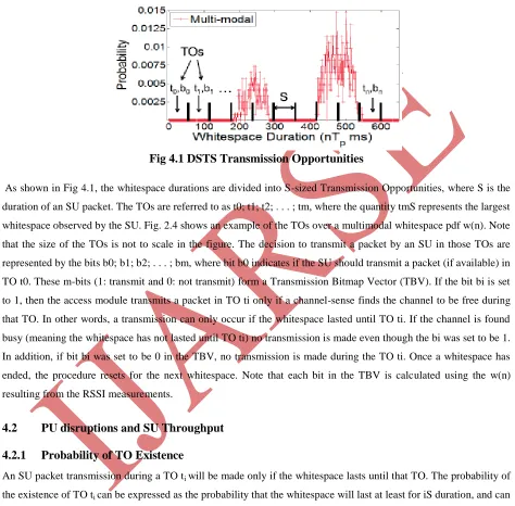
The key idea behind DSTS is for an SU to determine the best transmission opportunities as a function of the elapsed time in a whitespace.

Fig 4.1 DSTS Transmission Opportunities

As shown in Fig 4.1, the whitespace durations are divided into S-sized Transmission Opportunities, where S is the duration of an SU packet. The TOs are referred to as t0; t1; t2; . . . ; tm, where the quantity tmS represents the largest whitespace observed by the SU. Fig. 2.4 shows an example of the TOs over a multimodal whitespace pdf w(n). Note that the size of the TOs is not to scale in the figure. The decision to transmit a packet by an SU in those TOs are represented by the bits b0; b1; b2; . . . ; bm, where bit b0 indicates if the SU should transmit a packet (if available) in TO t0. These m-bits (1: transmit and 0: not transmit) form a Transmission Bitmap Vector (TBV). If the bit bi is set to 1, then the access module transmits a packet in TO ti only if a channel-sense finds the channel to be free during that TO. In other words, a transmission can only occur if the whitespace lasted until TO ti. If the channel is found busy (meaning the whitespace has not lasted until TO ti) no transmission is made even though the bi was set to be 1. In addition, if bit bi was set to be 0 in the TBV, no transmission is made during the TO ti. Once a whitespace has ended, the procedure resets for the next whitespace. Note that each bit in the TBV is calculated using the w(n) resulting from the RSSI measurements.

4.2

PU disruptions and SU Throughput

4.2.1

Probability of TO Existence

An SU packet transmission during a TO ti will be made only if the whitespace lasts until that TO. The probability of

the existence of TO ti can be expressed as the probability that the whitespace will last at least for iS duration, and can

be written as:

P

= 1-W(iS/T

)

(1)

where W(n) is the cumulative distribution function (cdf) of the whitespace pdf w(n), which is expressed as a multiple of the channel sensing interval Tp. When the bit bi is set to 1 in the TBV, the probability Piexistence will

determine if an SU transmission in TO ti will actually be possible or not. The Pi existence

probability will occur with greater frequency, thus resulting in higher SU throughput.

4.2.2

Probability of Disruption

An SU packet transmission during a TO tiwill cause a PU traffic disruption if the current whitespace does not last

for a full S duration since the start of the transmission. The probability of disruption is expressed as the probability that a whitespace lasts anywhere between (i-1)S to iS duration, and can be written as

P

= W(iS/T

) - W((i-1)S/T

)

(2)

Now consider a situation in which a specific TBV, T^ is selected. Let δ represent a subset (of all m bits in T^) of bits that are 1. The rest of the bits are set to 0. During a whitespace, after an SU transmits based on T^, the resulting Primary Traffic Disruption can be expressed as

PTD = ∑

P

(3)

4.3

Performance under Dynamic PU Traffic Patterns

Initially, the PU traffic is generated with 60 ms interpacket time (IPT) with the Uniform profile. The pattern changes after 60 seconds when the IPT is increased to 120 ms. Finally, at 100 seconds the IPT is changed to Poisson distribution with 90 ms average. The whitespace w(n) is continually computed by the access protocol after collecting every 1,000 whitespace samples. Observe that while the primary user traffic pattern changes over time, the PTDs resulting from the CSTS and DSTS access strategies stay consistently within the vicinity of the preset disruption bound of 0.05. Also, note that there is very little PU traffic disruption during the transitions of w(n) as indicated in both the frames. This is primarily because the whitespace pdf for ad hoc mode 802.11 traffic maintains very similar properties across different traffic patterns, i.e., above 90 percent of the whitespaces are below 1 ms.

Note that the SU throughput increases after a PU traffic pattern transition when the useable whitespace increases due to the increase in interpacket interval of the PU traffic. Additionally, the SU dynamically throttles back its transmissions to protect the PUs when the available whitespace reduces during a transition. These results demonstrate the robustness of the CSTS and DSTS access strategies against varying data rates over time. Additionally, the results suggest that by periodically measuring the channel state the SUs are able to dynamically model the channel whitespace and adjust their access parameters accordingly to minimize the PU disruptions and to maximize the SU throughput.

V JiST/SWANS

5.1

SWANS

SWANS is a complete library for simulation of MANETs running on the JiST engine. As already described in the introduction, MANET simulations need a model for the environment and for the nodes. In SWANS, the Field entity provides node mobility and radio propagation. Nodes consist of a number of entities implementing various protocol layers, where the radio entity is connected to the global field entity. Packets traverse the protocol stack entities usually as simple references, at virtually no cost. Duplication is only done where necessary, e.g. if a packet is broadcasted and needs to be changed by the forwarders. Regarding radio propagation, one can choose a free space or a two-ray-ground pathloss model, together with Rayleigh fading, Rician fading or without fading. Moreover, a statistic packet dropping can be applied. As node mobility, the standard distribution supplies teleporting, random walk and random waypoint models. For the composition of nodes, SWANS brings basic radio noise models, an implementation of 802.11b MAC, IPv4, AODV, DSR and ZRP MANET routing, as well as TCP and UDP transport and several applications. As a special feature, SWANS also allows to run legacy Java network applications as part of simulations.

5.2

Performance

When designing a new simulation tool, evaluation of performance is a primary concern. Performance evaluations have been conducted by the authors of JiST/SWANS in [3], specifically regarding the performance of the JiST engine, but also including SWANS simulations. For the JiST benchmark, a small simulation similar to the above example in Listing 1 was carried out. The program schedules an identical event step by step for 5 million times, so that only the raw event throughput is relevant. Then, the authors compare the runtime behavior with the same small program implemented in ns-2 and GloMoSim. As result of this competition, JiST performed this task 1:97 times faster than Parsec, 3:36 times faster than the ns-2 program (when implemented completely in C-code), 9:84 times faster than GloMoSim, and even 78:97 times faster than an ns-2implementation in Tcl. As a performance baseline, the authors also implemented a plain C program that imitates the scheduler behavior by inserting and removing elements from an eficient array-based priority queue. Compared to that, JiST performs 31% slower. Regarding memory consumption, JiST performs similarly well.

5.3

Ongoing efforts

Since the publication of JiST/SWANS, more and more researchers have started to use, to improve and to extend it. One of the earlier available extensions was STRAW [5], the "Street Random Waypoint" mobility model for simulation of vehicles driving on roads. Currently, this activity has been extended to an open source project called SWANS++. In addition, also numerous researchers have used JiST/SWANS in their work.

VI SPECIFICATIONS USED

6.1

Field Entity

In SWANS, the Field entity provides node mobility and radio propagation. Nodes consist of a number of entities implementing various protocol layers, where the radio entity is connected to the global field entity. Packets traverse the protocol stack entities usually as simple references, at virtually no cost. Here the node mobility is set as the random one. The radio propagation is a two-ray ground reflection model- A single line-of-sight path between two mobile nodes seldom the only means of propagation. The two-ray ground reflection model considers both the direct path and a ground reflection path. It is shown that this model gives more accurate prediction at a long distance than the free space model.

6.2

Routing Protocol

The routing technique used here is AODV routing. It is a reactive routing protocol, meaning that it establishes a route to a destination only on demand. In contrast, the most common routing protocols of the Internet are proactive, meaning they find routing paths independently of the usage of the paths. AODV is, as the name indicates, a distance-vector routing protocol. AODV avoids the counting-to-infinity problem of other distance-vector protocols by using sequence numbers on route updates, a technique pioneered by DSDV. AODV is capable of both unicast and multicast routing.

6.2.1

Working

In AODV, the network is silent until a connection is needed. At that point the network node that needs a connection broadcasts a request for connection. Other AODV nodes forward this message, and record the node that they heard it from, creating an explosion of temporary routes back to the needy node. When a node receives such a message and already has a route to the desired node, it sends a message backwards through a temporary route to the requesting node. The needy node then begins using the route that has the least number of hops through other nodes. Unused entries in the routing tables are recycled after a time.

number that limits how many times they can be retransmitted. Another such feature is that if a route request fails, another route request may not be sent until twice as much time has passed as the timeout of the previous route request.

The advantage of AODV is that it creates no extra traffic for communication along existing links. Also, distance vector routing is simple, and doesn't require much memory or calculation. However AODV requires more time to establish a connection, and the initial communication to establish a route is heavier than some other approaches.

6.2.2

Technical Description

The AODV Routing protocol uses an on-demand approach for finding routes, that is, a route is established only when it is required by a source node for transmitting data packets. It employs destination sequence numbers to identify the most recent path. The major difference between AODV and Dynamic Source Routing (DSR) stems out from the fact that DSR uses source routing in which a data packet carries the complete path to be traversed. However, in AODV, the source node and the intermediate nodes store the next-hop information corresponding to each flow for data packet transmission. In an on-demand routing protocol, the source node floods the RouteRequest

packet in the network when a route is not available for the desired destination. It may obtain multiple routes to different destinations from a single RouteRequest. The major difference between AODV and other on-demand routing protocols is that it uses a destination sequence number (DestSeqNum) to determine an up-to-date path to the destination. A node updates its path information only if the DestSeqNum of the current packet received is greater or equal than the last DestSeqNum stored at the node with smaller hopcount.

A RouteRequest carries the source identifier (SrcID), the destination identifier (DestID), the source sequence number (SrcSeqNum), the destination sequence number (DestSeqNum), the broadcast identifier (BcastID), and the

VII EXPERIMENTAL RESULT ANALYSIS

Observe in Fig. 7.1 that while the PU traffic pattern changes over time, the PTD resulting from DSTS stays consistently within the vicinity of the DB of 0.05.

Fig. 7.1 Output for channel sensing period versus Primary user Traffic Disruption

Fig. 7.2 Output for Channel Sensing Period versus Effective Secondary user Throughput

Also, observe that there is very little PTD during the transitions of the PU traffic patterns as indicated in both the frames in Fig. 7.1 and 7.2. This is mainly because the whitespace pdf for Ad-hoc mode 802.11 traffic has very similar properties across different traffic patterns, i.e. above 90% of the whitespace is below 1 ms (see Fig. 3.1). The SU throughput increases during a traffic pattern transition if the useable whitespace increases due to the increase in IPT of the PU traffic. Additionally, the SU dynamically throttles back its transmissions to protect the PUs when the traffic change reduces the available amount of whitespace. These results show the robustness of DSTS against varying topologies and data rates in the primary network over time.

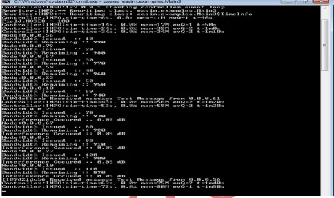
In this paper, we can set maximum of more than 1000 nodes using the JiST/SWANS software. It could be set while simulating the experiment. Two cases were depicted in this project - wired and wireless adhoc.

The nodes are set by clicking the tools menu on the top corner of the easim window. After setting the nodes, the mobility of those nodes will be started by right clicking on the page displayed. After starting the mobility, the client node is set first and then the server node.

After setting the server node, simulation starts. The output shows the number of nodes the data has crossed to reach the client node from the server node. The nodes through which the data will be transmitted will be selected using shortest path method. Also bandwidth used by each node to transmit the data and bandwidth remaining will be displayed.

The interference occurred while transmitting the data for the first time of transmission will be zero, which could be taken as the Primary User transmission. In the subsequent transmissions, there is a possibility of interference to occur, which could also be displayed in the result. This interference increases with increase in the number of data to be transmitted i.e., when the packet size of the data increases, interference to the PU transmission increases.

0 0.01 0.02 0.03 0.04 0.05 0.06

0 0.1 0.2 0.3 0.4 0.5 0.6 0.7 0.8 0.9 1

TOP 1, P 60 TOP 2, U 70 TOP 3, U 70

Sensing Period Tp

(ms) P T D 0.82 0.83 0.84 0.85 0.86 0.87 0.88 0.89 0.9 0.91 0.92

0 0.1 0.2 0.3 0.4 0.5 0.6 0.7 0.8 0.9 1

TOP 1, P 60

TOP 2, U 70

TOP 3, U 70

Sensing Period Tp (ms)

Fig. 7.3 Simulated output of the scenario created in JiST/SWANS

Thus in the output, the values of bandwidth used, bandwidth remaining, interference occurred and nodes through which data are transmitted are displayed, which are the result of the scenario created using JiST/SWANS software.

VIII CONCLUSIONS

Thus from the above theoretical results, it has been concluded that if we use DSTS, the disruption to the primary users will be very low in the range of 5% with very high secondary user throughput. From the simulation result, a scenario of MANET has been described using JiST/SWANS with any number of user-defined nodes.

As further enhancement, we shall use SWANS++, an emerging simulator to depict the scenario for the dynamic spectrum access. In this project, the data to be transmitted is taken as the text messages sent through Internet Messenger. The same scenario could be depicted for audio messages like voice chat.

ACKNOWLEDGEMENT

REFERENCES

[1] A. Plummer Jr., M. Taghizadeh, S. Biswas, “Measurement-Based Bandwidth Scavenging in Wireless Networks”, IEEE CS, CASS, ComSoc, IES, & SPS, Jan. 2012.

[2] R. L. Bagrodia, R. Meyer, M. Takai, Y. Chen, X. Zeng, J. Martin, and H. Y. Song. Parsec: A parallel simulation environment for complex systems. IEEE Computer, 31(10):77-85, Oct. 1998.

[3] R. Barr and Z. J. Haas. JiST/SWANS website, 2004. http://www.cs.cornell.edu/barr/repository/jist/. [4] S. Geirhofer, L. Tong, and B.M. Sadler, “Dynamic Spectrum Access in WLAN Channels: Empirical Model

and Its Stochastic Analysis,” Proc. First Int’l Workshop Technology and Policy for Accessing Spectrum (TAPAS ’06), 2006.

[5] R. M. Fujimoto. Parallel discrete event simulation: Will the field survive? ORSA Journal on Computing, 5(3):213-230, 1993.

[6] R. M. Fujimoto. Parallel and distributed simulation. In Winter Simulation Conference, pages 118-125, Dec. 1995.

[7] S. Geirhofer, L. Tong, and B.M. Sadler, “Cognitive Medium Access: Constraining Interference Based on Experimental Models,” IEEE J. Selected Areas in Comm., vol. 26, no. 1, pp. 95-105, Jan. 2008.

[8] S. Huang, X. Liu, and Z. Ding, “Optimal Transmission Strategies for Dynamic Spectrum Access in Cognitive Radio Networks,” IEEE Trans. Mobile Computing, vol. 8, no. 12, pp. 1636-1648, Dec. 2009. [9] D. M. Nicol. Parallel discrete event simulation: So who cares? In Workshop on Parallel and Distributed

Simulation, June 1997.

[10] D. M. Nicol and R. M. Fujimoto. Parallel simulation today. Annals of Operations Research, pages 249-285, Dec. 1994.

[11] B. Wang, Z. Ji, and K.J. Ray Liu, “Primary-Prioritized Markov Approach for Dynamic Spectrum Access,”

Proc. IEEE Int’l Symp. New Frontiers in Dynamic Spectrum Access Networks (DySPAN ’07), 2007.

[12] G. Riley and M. Ammar. Simulating large networks: How big is big enough? In Conference on Grand Challenges for Modeling and Sim., Jan. 2002.

[13] S. Huang, X. Liu, and Z. Ding, “On Optimal Sensing and Transmission Strategies for Dynamic Spectrum Access,” Proc. IEEE Third Symp. New Frontiers in Dynamic Spectrum Access Networks (DySPAN ’08),

2008.

[14] "Overview of Wireless Communications"

www.cambridge.org/us/catalogue/catalogue.asp?isbn=0-521-83716-2&ss=exc. Retrieved 2008-02-08. [15] "Wireless Network Industry Report". http://