Faults: A Machine Learning Approach
Sayandeep Saha1, Dirmanto Jap2, Sikhar Patranabis1, Debdeep Mukhopadhyay1,
Shivam Bhasin2, and Pallab Dasgupta1
1 Department of Computer Science and Engineering, IIT Kharagpur, India 2
Physical Analysis & Cryptographic Engineering (PACE) Labs, Nanyang Technological University, Singapore
E-mail:{sahasayandeep,sikhar.patranabis,debdeep, pallab}@cse.iitkgp.ernet.in,{djap,sbhasin}@@ntu.edu.sg
Abstract. Characterization of the fault space of a cipher to filter out a set of faults potentially exploitable for fault attacks (FA), is a prob-lem with immense practical value. A quantitative knowledge of the ex-ploitable fault space is desirable in several applications, like security evaluation, cipher construction and implementation, design, and test-ing of countermeasures etc. In this work, we investigate this problem in the context of block ciphers. The formidable size of the fault space of a block cipher mandates the use of an automation to solve this prob-lem, which should be able to characterize each individual fault instance quickly. On the other hand, the automation is expected to be applicable to most of the block cipher constructions. Existing techniques for au-tomated fault attacks do not satisfy both of these goals simultaneously and hence are not directly applicable in the context of exploitable fault characterization. In this paper, we present a supervised machine learning (ML) assisted automated framework, which successfully addresses both of the criteria mentioned. The key idea is to extrapolate the knowledge of some existing FAs on a cipher to rapidly figure out new attack instances on the same. Experimental validation of the proposed framework on two state-of-the-art block ciphers – PRESENT and LED, establishes that our approach is able to provide fairly good accuracy in identifying exploitable fault instances at a reasonable cost. Finally, the effect of different S-Boxes on the fault space of a cipher is evaluated utilizing the framework.
1
Introduction
today. However, it has been shown on several occasions that albeit being mathe-matically secure, unless properly implemented and protected, such cryptographic cores may lead to catastrophic security vulnerabilities by leaking secrets to ma-licious parties. In particular, one must ensure the cryptographic security of the primitives against implementation specific attacks like passive side channel anal-ysis and active fault attacks, which have recently gained a lot of attention from both industry and academia, due to their practicality and diversity.
Fault-based cryptanalysis or Fault Attacks (FA) is a class of active imple-mentation based attacks, which typically exploit transient faults in the data and/or control paths of a cipher during its execution to extract the secret key. Among different sub-classes of FA, Differential Fault Analysis (DFA) attacks are particularly interesting in the context of block ciphers, due to their low data/fault complexity and easy-to-mount nature. In DFA, the adversary injects faults with certain known spatiotemporal characteristics and then analyzes the pairs of faulty and the corresponding fault-free ciphertexts to recover the secret key. It is well established that even a single properly placed malicious fault is able to compromise the security of mathematically strong block ciphers in cer-tain cases. One prominent example of this fact is the AES [1], where a random byte fault at the 8th round of the cipher can compromise the 128-bit secret key [2].
Given a block cipher, the discovery of a DFA attack is, however, nontrivial, as not all possible faults may lead to successful attacks. Traditional approaches for DFAs are mostly manual and demand special expertise on cryptanalysis. Till date, numerous block ciphers have been designed and deployed in-field for vari-ous applications [1,3]. Moreover, there is a growing trend of designing application and platform-specific lightweight ciphers, tailored for resource-constrained envi-ronments [4, 5]. Recently, NIST has launched an international competition to standardize lightweight cryptographic primitives. It is quite apparent that thor-ough analysis of such a large number of ciphers is impractical with manual DFA techniques and therefore automated DFA tools must be devised for this purpose. Further, such automated tools should work with minimal manual intervention and must be applicable to a large class of block ciphers and fault models.
Recently, there have been significant advances in designing such tools [6– 11]. The most prominent among these automated frameworks is the so-called Algebraic Fault Attack (AFA), which encodes a given cipher and an injected fault as a system of multivariate polynomial equations on the finite fieldGF(2) in Algebraic Normal Form (ANF) [6–10]. The ANF system is then converted to an equivalent system in Conjunctive Normal Form (CNF) and fed to a Boolean Satisfiability (SAT) solver with the aim of extracting the key by solving the system.
faults. The knowledge of the exploitable fault space might also be desired for designing ciphers with some inherent fault attack resilience, testing of counter-measures, and guided synthesis of countermeasures for resource-constrained en-vironments. However, the formidable size of the fault spaces usually encountered in block ciphers makes the problem of exploitable fault space characterization much more difficult than finding individual DFAs. Typically, a fault instance in a cryptographic primitive depends on different aspects (e.g. the location, the width of the fault, the mathematical structure of the cipher, and the number of times a fault is injected) and consideration of each of these aspects results in a fault space of prohibitive size, which may be hard to enumerate. Even a statistical characterization of this fault space is difficult and one must obtain a sufficiently large number of samples, as the distribution of the fault space may be unknown, even for well-studied ciphers.
The very nature of the exploitable fault characterization problem demands an automated solution for this purpose. From the perspective of a cipher designer or system architect, the characterization process for each individual fault should be fast enough so that significant fraction of the fault space can be covered within a reasonable time. Another desirable requirement for such automation is that it must be generic enough for the large class of existing and future cipher designs. Unfortunately, none of the automated fault attack frameworks proposed till date satisfy both these criteria, simultaneously. In particular, the AFA, which is fairly generic in nature, involves solving a SAT problem for each individual fault instance. Although SAT solvers are remarkably good at finding solutions to a large class of NP-Complete problem instances, the time taken for solving is often prohibitively high. In fact, in the context of AFA attacks, the solver may not stop within a reasonable time for many fault instances. Although, setting a proper timeout seems to be a reasonable fix for such cases, the variation of solving times is often very high and as a result, the timeout threshold must be reasonably high as well, to guarantee the capture of every possible attack. It is thus quite evident that exhaustive analysis of the fault space by means of AFA is impractical as far as the time is concerned.
1.1 Our Contributions
The contributions of this paper are as follows:
– The proposed framework is experimentally evaluated on two state-of-the-art lightweight block ciphers – PRESENT [4] and LED [5]. In particular, we show that ML models can predict new attack instances for a block cipher with significantly high accuracy, while being trained with a reasonably small number of known attack instances on the same.Specifically, we obtain
training accuracies of 85 - 93% in our experiments.Further, we
pro-pose a simple strategy to nullify the risk of misclassifying exploitable faults as benign ones, which is found to work fairly well for our case studies.Our experiments establish that the false negatives can be nullified by exhaustively testing roughly 20% of the total fault samples, which is quite reasonable. Further, it is found that the ML models can predict difficult attack instances while trained on a set of relatively easier attack instances, which is indeed a remarkable result, so far the capability of the tool is concerned.
– In order to establish the importance of exploitable fault characterization, we present an application scenario, which sheds light on a previously unex-plored effect of non-linear layers on the exploitable fault space of a block cipher. We study the effect of 3 structurally similar S-Boxes in the context of DFA attacks on bit-permutation based SPN ciphers. The experiments were performed for PRESENT, which is the most prominent member of this class. It is found that the statistical characterization of exploitable fault space provides interesting information about the effect of non-linear layers in the context of DFAs.In particular, we observe that the S-Box of SKINNY [43] is relatively more resistant to DFAs than the S-Boxes of PRESENT and SERPENT [3].
The rest of the paper is organized as follows. In the next section, we present a brief overview of fault-based cryptanalysis with an emphasis on automated fault analysis techniques. Some necessary preliminaries are presented in Section 3. We elaborate the proposed framework in Section 4, along with supporting case studies and a potential application scenario in Section. 5. Concluding remarks are presented in Section 6.
2
Background
In this section, we outline the necessary backgrounds on fault attacks with an emphasis towards automated fault analysis. We begin with a brief introduction to fault analysis attacks on block ciphers. The AFA and some other approaches for automated fault attacks will be summarized next with emphasis on the concepts relevant for this work.
2.1 Fault Attacks on Block Ciphers: A Brief Survey
The concept of Differential Fault Analysis (DFA) was introduced by Biham et. al. [14] on the Data Encryption Standard (DES), and was readily adapted for other ciphers like AES [1], PRESENT [4], LED [5] etc. In particular, AES is the most extensively studied cipher in the context of fault attacks [2,15–19]. The ba-sic principle of any fault attack is to cause a malicious aberration in the normal execution of the target cryptographic algorithm and to exploit the corresponding leakage to try and recover the secret key within reasonable computational com-plexity. Till date, DFAs are the most widely studied class of fault attacks. DFAs, in general, exploit computationally efficient key distinguishers resulting from the fault injection and recover the secret key by solving a system of equations con-structed with the distinguishers. The existence of practically achievable fault models such as bit faults, nibble faults, byte faults, and diagonal faults makes DFA a potent threat for modern block ciphers.
Although DFA constitutes the most prominent class of fault attacks, there exist other variants which have recently gained significant attention mainly due to their simplicity. Differential Fault Intensity Analysis (DFIA) is a non-DFA technique [20, 21]. DFIA combines the concept of side-channel analysis with fault attack to recover the secret key by exploiting the faulty ciphertexts only. However, the number of required ciphertexts are significantly higher than in DFA. The Safe-Error Attacks (SEA), Differential Behaviour Analysis (DBA) and Fault Sensitivity Analysis (FSA) constitute the other major categories of fault attacks. The main crux of these attacks lies in the fact that depending on a particular sub-part of the secret key (such as a bit or a byte), a fault may or may not lead to a faulty computation. The very presence of a fault in a computation thus leaks critical information which leads to the extraction of the key [19, 22]. It should be noted that all these attacks including DFIA are statistical in nature and their success critically depends on the physical characteristics of the target implementation.
2.2 Automated Fault Analysis
off-the-shelf SAT solvers for solving. Perhaps the most attractive feature of AFA is its genericness. In [10], Zhang et. al. have shown that the algebraic framework can encode most of the DFA like attacks including the attacks on key schedule and round counters. Moreover, it has been anticipated that AFA are powerful than conventional DFA in certain situations as they can exploit many equations which are otherwise beyond the perception of a human attacker [10]. All such features of AFA make it the perfect candidate for automated fault analysis.
Recently, Khanna et. al. [11] has proposed a novel approach for automated fault analysis called XFC, which is significantly different from the AFA approach. Through a coloring based abstraction, XFC first enumerates the fault propaga-tion path of a cipher and then calculates the complexity of the key space which is expected to be reduced significantly, if a fault is exploitable. The computation procedure of XFC is fairly simple and fast compared to the AFA approaches, which makes it a potential candidate for exploitable fault characterization. How-ever, the framework is found to be restricted to a very specific class of DFA and also lacks proper automation. Barthe et. al. [12] has proposed another alternative approach for public key algorithms where, the vulnerable locations in a software implementation are identified for a given attack condition using program syn-thesis techniques. However, it requires prior knowledge of the fault conditions. Also the program synthesis is not known to be a very fast approach in general.
3
Preliminaries
3.1 General Model for Block Cipher and Faults
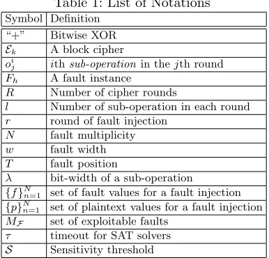
Table 1: List of Notations Symbol Definition
“+” Bitwise XOR
Ek A block cipher
oi
j ithsub-operationin thejth round
Fh A fault instance
R Number of cipher rounds
l Number of sub-operation in each round
r round of fault injection
N fault multiplicity
w fault width
T fault position
λ bit-width of a sub-operation
{f}N
n=1 set of fault values for a fault injection {p}N
n=1 set of plaintext values for a fault injection
MF set of exploitable faults τ timeout for SAT solvers
Let Ek be a block cipher defined as a tuple Ek = hEnc, Deci, where Enc
andDec denote the encryption and decryption functions, respectively. Further, theEncfunction (and similarly theDecfunction) is defined as Enc(p) =AR◦
AR−1◦...◦ A1(p) = c, for a plaintext p ∈ P, ciphertext c ∈ C, and a key
k ∈ K. EachAj denotes a round function in a Rround cipher. Further, each
Aj = olj ◦o l−1
j ◦...◦o1j is a composition of certain functions of the form oij,
generally denoted as sub-operations in this work. EachAj is thus assumed to
have l sub-operations. A sub-operation may belong to the key schedule or the datapath of the cipher. In other words, oij denotes either a key schedule sub-operation or a datapath sub-sub-operation at any roundj. We shall use the termoij
throughout this work to denote a sub-operation, without mentioning whether it belongs to key schedule or datapath. Table. 1 lists the notations used throughout this paper.
An injected fault in DFA usually corrupts the input of some specific sub-operation during the encryption or decryption sub-operation of the cipher. Given the cipher model, we denote the set of faults as F = {F1, F2, ..., FH}, where
each individual faultFh∈ F is specified as follows:
Fh=hoir, λ, w, T, N,{f} N n=1,{p}
N
n=1i (1)
Here r < R is the round of injection, and oi
r denotes the sub-operation,
in-put of which is altered with the fault. The parameterλdenotes the data-width of the operation (more specifically, the bit-length of the input of the sub-operation). The parameterwis the width of the fault which quantifies the max-imum number of bits affected by a fault. In general,bit-based,nibble-based, and
byte-based fault models are considered which corresponds to w =1, 4, and 8,
respectively. Theposition of the fault at the input of a sub-operation is denoted byT witht∈ {0,1, ...wλ}. For practical reasons,wandT are usually defined in a way so that the injected faults always remain localized within some pre-specified block-operations of the corresponding sub-operation oi
r. The parameter N
rep-resents the number of times, a fault is injected at a specific location to obtain a successful attack within a reasonable time.N is called theFault Multiplicity.
The sets{f}N
n=1, and{p}
N
n=1 denote the values of the injected faults and the plaintexts processed during each fault injection, respectively. In the most general case, the diffusion characteristics (and thus the exploitability) of an injected fault critically depends upon the value of the fault and the corresponding plaintext on which the fault is injected. A typical example is PRESENT cipher, where, the number of active S-Boxes due to the fault diffusion depends on the plaintext and the fault value and as a result, many faults injected at a specific position with the same multiplicity may become exploitable, whereas some of them at the same position may become unexploitable. According to the fault model in Equation 1, the total number of possible faults for a specific positionT in sub-operationoi
ris 2N(w+λ), for a given fault widthw. The total number of possible
faults for a sub-operationoi
r is 2N(w+λ)×
λ w
, and that for the whole cipher is
oi
r is 2N(w+λ)×
λ
w×R×l
In certain cases the fault space can be pruned significantly utilizing the fact that a large number of faults may be actually equivalent. A prominent example is the AES where every byte fault at some specific position is equivalent irrespective of its value. However, there exists no automatic procedure to figure out such equivalences, till date, and the only way is to manually analyze the cipher. As a result, it is reasonable to adapt the above calculation of the size of the fault space while analyzing a general construction.
3.2 Algebraic Representation of Ciphers
Multivariate polynomial representation, which is quite well-known in the context of AFA [10], is considered one of the most generic and informative representations for block ciphers. In this work, we utilize the polynomial representations to encode both the ciphers and the faults. The usual way of representing block ciphers algebraically is to assign a set of symbolic variables for each iterative round, where each variable represents a bit from some intermediate state of the cipher. Each cipher sub-operation is then represented as a set of multivariate polynomial equations over the polynomial ring constructed on these variables, with GF(2) being the base ring. The equation system should be sparse and low-degree in addition, to make the cipher representation easy to solve.
In order to elaborate the process of polynomial encoding, we consider the example of the PRESENT block cipher. PRESENT is a lightweight block ci-pher proposed by Bogdanov et. al. in CHES 2007 [4]. It has a Substitution-Permutation Network (SPN) based round function which is iterated 31 times to generate the ciphertext. The basic version PRESENT-80 has a block size of 64-bits and a master key of size 80 bits, which is utilized to generate 64-bit round keys for each round function by means of an iterated key-schedule. Each round of PRESENT consists of three sub-operations, namely, addRoundKey, sBoxlayer,
andpLayer. TheaddRoundKey sub-operation, computing bitwise XOR between
the state bits and round key bits is represented as:
yi=xi+ki, for 1≤i≤64 (2)
where,xi,kirepresents the input state bits and round key bits, respectively, and
yi represents the output bits of theaddRoundKey sub-operation. Similarly, the
pLayer operation, which is a 64-bit permutation can be expressed as:
yπ(i)=xi, for 1≤i≤64 (3)
whereπ(i) is the permutation table. The non-linear substitution operationsBoxlayer
of PRESENT consists of 16 identical 4×4 bijective S-Boxes, each of which can be represented by a system of non-linear polynomials. The solvability of a typical cipher polynomial system critically depends on the S-Box representation, which is expected to be sufficiently sparse and consisting of low-degree polynomials. One way of representing the PRESENT S-Boxes is the following:
y1=x1x2x4+x1x3x4
y2=x1x2x4+x1x3x4+x1x3+x1x4+
x1+x2+x3x4+ 1
(4)
y3=x1x2x4+x1x2+x1x3x4+x1x3+
x1+x2x3x4+x3
y4=x1+x2x3+x2+x4
Here xis (1≤i≤4) andyis (1≤i≤4) represent the input and output bits of
a 4×4 S-Box, respectively.
Each injected fault instance can be added in the cipher equation system in terms of new equations. Let us assume that the fault is injected at the input state of theith sub-operationoi
r at therth round of the cipher. For convenience, we
denote the input ofoi
r asXi=x1||x2||...||xλ, whereλis the bit-length ofXi. In
the case of PRESENTλ= 64. Let, after the injection of the fault, the input state changes toYi=y1||y2||...||yλ. Then the state differential can be represented as
Di =d1||d2...||dλ, wheredz =xz+yz with 1≤z < λ. Further, depending on
the width of the fault w, there can be m= wλ possible locations in Xi, which might have got altered. Let us partition the state differential Di in m, w-bit
chunks as Di = Di
1||Di2||...||Dmi , where Dit = dw×(t−1)+1||dw×(t−1)+2||...||dw×t
for 1≤t≤m. AssumingT be the location of the fault, the fault effect can be modelled with the following equations:
Dit= 0, for 1≤t≤m, t6=T (5)
(1 +dw×(t−1)+1)(1 +dw×(t−1)+2)...(1+dw×t) = 0,
fort=T (6)
It is notable that the locationT of a fault can be unknown in certain cases, and this can also be modeled with equations of slightly complex form [10]. However, for exploitable fault characterization, it is reasonable to assume that the locations are known as we are working in the evaluator mode.
4
Proposed Methodology
4.1 Motivation
The goal of the present work is to efficiently filter out the exploitable faults for a given cryptosystem. It is apparent that the ANF polynomials provide a reasonable way for modeling the ciphers and the faults [10]. Although, the ANF description and its corresponding CNF is easy to construct, solving them is non-trivial as the decision problem associated with the solvability of an ANF system is NP-Complete. In practice, SAT solvers are used for solving the associated CNF systems and it is observed that the solving times vary significantly depending on the instance.
pair there always exists a key. However, it is not practically feasible to figure out the key without fault injections, as the size of the key search space is prohibitively large. The search space complexity reduces with the injection of faults. The size of the search space is expected to reach below some certain limit which is possible to search exhaustively with modern SAT solvers within reasonable time, if a sufficient number of faults are injected at proper locations.
The above-mentioned observation clearly specifies the condition for distin-guishing the exploitable faults from the non-exploitable ones. To be precise, if a SAT solver terminates with the solution within a prespecified time limit, the fault instance is considered to be exploitable. Otherwise, the fault is considered non-malicious. Setting a proper time-limit for the SAT solver is, however, a crit-ical task. A relatively low time-limit is unreliable as it may fail to capture some potential attack instances. As an example, for the PRESENT cipher we observed that most of the 1-bit fault instances with fault multiplicity 2, injected at the inputs of 28-th round S-Box operation, are solvable within 3 minutes. This ob-servation is similar to that mentioned in [10]. However, we observed that when nibble faults are considered at the 28th round, the variation of solving time is sig-nificantly high; in fact, there are cases with solving times around 16−24 hours. These performance figures are obtained with Intel Core i5 machines running CryptominiSAT-5 [33] as the SAT solver in a single threaded manner. Moreover, such cases comprise nearly 12% of the total number of samples considered. This is not insignificant in a statistical sense, where failure in detecting some attack instances cannot be tolerated. Such instances do not follow any specific pattern through which one can visually characterize them without solving them. This observation necessarily implies that one has to be more careful while setting solver timeouts and a high value of timeout is preferable. However, setting high timeout limits the number of instances one can acquire through exhaustive SAT solving within a practically feasible time span.
4.2 Empirical Hardness Prediction of Satisfiability Problems
NP-Complete problems are ubiquitous in computer science, especially in AI. While they are hard-to-solve on worst case inputs, there exists numerous “easy” instances which are of great practical value. In general, the algorithms for solving NP-Complete problems exhibit extreme runtime variations even across the solv-able instances and there is no describsolv-able relationship between the instance size and the algorithm runtime as such. Over the past decade, a considerable body of work has shown how to use supervised ML models to answer questions regard-ing solvability or runtime usregard-ing features of the problem instances and algorithm performance data [24–28]. Such ML models are popularly known as Empirical Hardness Models (EHM). Some applications of EHMs include proper algorithm portfolio selection for a problem instance [28], algorithm parameter tuning [25], hard benchmark construction [29], and analysis of algorithm performance and instance hardness [29].
In the context of the present work, we are interested in EHMs which pre-dict the hardness of SAT instances. The most prominent result in the context of empirical runtime estimation of SAT problems is due to Xu et. al., who con-structed a portfolio based SAT solver SATzilla [28] based on EHMs. The aim of SATzilla was to select the best solver for a given SAT instance, depending upon the runtime predictions of different EHMs constructed for a set of representative SAT solvers. The SATzilla project also provided a large set of 138 features for the model construction depending on various structural properties of the CNF descriptions of the problem instance as well as some typical features obtained from runtime probing of some basic SAT solvers. In this work, we utilize some of these features for constructing EHMs which will predict the exploitability of a given fault instance without solving it explicitly. Brief description of our feature set will be provided later in this section.
4.3 ML Model for Exploitable Fault Identifier
In this subsection, we shall describe the ML-based framework in detail. In nut-shell, our aim is to construct a binary classifier, which, if trained with certain number of exploitable and unexploitable fault instances, can predict the ex-ploitability of any fault instance queried to it. Before going to further details, we formally describe the exploitable fault space for a given block cipher and an exploitable fault in the context of SAT solvability.
Definition 1 (Exploitable Fault Space) Given a cipherEkand a
correspond-ing fault spaceF, the exploitable fault space MF ⊂ F forEk is defined as a set
of faults such that∀Fh∈MF, it is possible to extractne bits of the secret keyk,
where0< ne≤ |k| .
In other words, exploitable fault space denotes the set of faults for which the combination of the injected fault and a plaintext results in the extraction ofne
CipherEk Fault SpaceF=fF1; F2; :::; FHg
fAN F(EFh
k )g
Set of Fault induced Cipher Equations
Set of CNFs fCN F(EFh
k )g
Itr⊂fCN F(EFh
k )g
Get Runtimes via SAT Solving
Extract CNF Features (T(Itr)) and Label with Runtimes
fCN F(EFh
k )g nItr
Verify Exploitability
MF⊂fCN F(EFh
k )g
1
2
3
4 Model Training
5 6
M
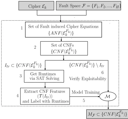
Fig. 1: The Exploitable Fault Characterization Framework: Basic Idea
of the key bits are known apriori and faults are inserted to extract the complete master key of the cipher. Indeed, one may increase the number of injections to reduce the complexity of the search space in this scenario. However, it is practically reasonable to assume some upper bound on the number of injections. In other words, the fault multiplicity N in the fault model is always ≤ some pre-specified threshold. The second scenario in this context occurs when some specific key bits are assumed to be known. This model is extremely useful when only a subset of the key can be extracted by the fault injection due to incomplete diffusion of the faults. In a typical AFA framework, it is not possible to obtain a unique solution for the incompletely defused faults unless some of the key bits are known. However, in this work, we mainly elaborate the first scenario. It is worth mentioning that, the second scenario can be dealt with the framework we are going to propose, without any significant changes.
The framework for exploitable fault space characterization is depicted in Figure. 1. Referring to the figure, let EFh
k indicate the cipher Ek, with a fault
Fh from its fault space F injected in it. This can be easily modelled as an
ANF equation system denoted as AN F(EFh
k ). The very next step is to convert
AN F(EFh
k ) to the corresponding CNF model denoted by CN F(E Fh
k ). At this
point, we specify the exploitable faults in terms of solvability of SAT problems, with the following definition:
Definition 2 (Exploitable Fault) A fault Fh ∈ F for the cipher Ek is called
exploitable if the CN F(EFh
k ) is solvable by a SAT solver within a pre-specified
time boundτ.
ex-haustively with SAT solver and labeled accordingly depending on whether they are solvable or not within the thresholdτ. Next, a binary classifierMis trained with these labeled instances, which is the EHM in this case. The ML model is defined as:
M:T(CN F(EFh
k ))7→ {0,1} (7)
Here,T is an abstract function which represents the features extracted from the CNFs. In the present context,T outputs the feature vectors from the SATzilla feature set [28]. For convenience, we use the following nomenclature:
Class 0 : Denotes the class of exploitable faults.
Class 1 : Denotes the class of benign/unexploitable faults.
One important difference of our EHM model with the conventional EHM models is that we do not predict the runtime of an instance but use the labels 0 and 1 to classify the faults into two classes. In other words, we solve a classifi-cation rather than a regression problem solved in conventional EHMs [27]. The reason is that we just do not exploit the runtime information in our framework. The main motive of ours is to distinguish instances whose search space size is within the practical search capability of a solver, from those instances which are beyond the practical limit. It is apparent that our classifier based construction is sufficient for this purpose. In the next section, we describe the feature set utilized for the classification.
4.4 Feature Set Description
In this work, we use the features suggested by the SATzilla – a portfolio based SAT solving tool [28]. The SATzilla project proposed a rich set of 138 features to be extracted from the CNF description of a SAT instances for the construction of runtime predicting EHMs. The feature set of SATzilla is a compilation of sev-eral algorithm-independent properties of SAT instances made by the Artificial Intelligence (AI) community on various occations [29]. A widely known exam-ple of such algorithm-independent properties is the so-called phase-transition
of random 3-SAT instances. In short, SAT instances, generated randomly on a fixed number of variables, and containing only 3-variable clauses, tend to become unsatisfiable as the clause-to-variable ratio crosses a specific value of 4.26 [24]. Intuitively, the reason for such a behavior is that instances with fewer clauses are underconstrained and thus almost always satisfiable, while those with many clauses are overconstrained and unsatisfiable for most of the cases. The SATzilla feature set is divided into 12 groups. Some of the feature groups consist of struc-tural features like the one described in the example, whereas the others include features extracted from runtime behaviors of the SAT instances on solvers from different genre – like Davis-Putnam-Logemann-Loveland (DPLL) solvers, or lo-cal search solvers [27, 28].
features based on complex clause-variable interactions in the CNF formula ob-tained through different graph-based abstractions. Intuitively, these statistical measurements somewhat quantify the difficulty of an instance. The so-called run-time features in SATzilla, also known as “probing” features, are computed with short-time runs of the instances on different genres of candidate solvers. The computation times for these 12 groups of features are not uniform and there exist both structural and runtime features which are computationally expen-sive. The computation time of the features also provide significant information regarding the instance hardness and as a result, they are included as the final feature group. Further details on the feature set can be found in [26, 27].
4.5 Handling the False Negatives:
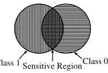
Class 0 Class 1 Sensitive Region
Fig. 2: Sensitive Region: Conceptual Illustration
The ML model proposed in this work provides quick answers regarding the exploitability of the fault instances queried to it. Such a quick answering system has an enormous impact on the exploitable characterization problem as it makes the problem tractable from a practical sense. However, the efficiency comes at the cost of accuracy. Being a ML-based approach, there will always be somefalse positives(a benign fault instance classified as exploitable) andfalse negatives(an exploitable instance classified as benign). While a small number of false positives can still be tolerated, false negatives can be crucial for some applications, for example, generating a test set of exploitable faults for testing countermeasures. If some typical exploitable faults are missed, they may lead to successful attacks on the countermeasure.
Determination of the sensitive instances or this region of overlap is, however, not straightforward and could be dealt in many ways. In this paper, we take a very simple albeit effective strategy. We useRandom Forest(RF) of decision trees as our classification algorithm [38]. Random forest is constructed with several decision trees, each of which is a weak learner. Usually, such ensemble methods
of learning performs majority voting among the decisions of the constituent weak learners (decision trees in the present context) to determine the class of the instance. Here, we propose a simple methodology for eliminating the false negatives using the properties of the RF algorithm. The proposed approach is reminiscent of classification with reject – a well-studied area in ML, where a classifier can reject some instances if the classification confidence is low for them [32]. Let Cl be the random variable denoting the predicted class of a given instance x in the two-class classification problem we are dealing with. For any instance x, we try to figure out the quantities P r[Cl = 0 | x] and
P r[Cl= 1|x], which are basically the probabilities ofxlying in any of the two classes. Evidently, the sum of these two quantities is 1. Note that the probabilities are calculated purely based on the decisions made by the classifier. In other words, it is calculated exploiting the properties of the classification algorithm. Next, we calculate the following quantity:
δ= (P r[Cl= 0|x]−P r[Cl= 1|x]) (8) It is easy to observe that having a large value for δ implies the classifier is reasonably confident about the class of the instancex. In that case, we consider the decision of the classifier as the correct decision. For the other case, where δ
is less than some predefined thresholdS, we invoke the SAT solver to determine the actual class of the instance. The overall flow for false negative removal is summarized in Algorithm 1.
Algorithm 1 ProcedureCLASSIF Y F AU LT S
Input: A random fault instanceFh Output: Exploitability status ofFh
1:ConstructAN F(EkFh) and thenCN F(EkFh)
2:Computex=T(CN F(EkFh))
3:ComputehP r[Cl= 0|x], P r[Cl= 1|x]i = M(x)
4:Computeδusing Equation (8)
5:if (|δ|<S)then .Sis a predefined threshold
6: Query the SAT engine withCN F(EFhk )
7: if (CN F(EkFh) is solvable withinτ)then 8: ReturnFh∈MF
9: else
10: ReturnFh6∈MF 11: end if
12: else
13: if(δ >0)then
14: Return0 . Fh∈MF
15: else
16: Return1 . Fh6∈MF
Each tree in an RF returns the class probabilities for a given instance. The class probability of a single tree is the fraction of samples of the same class in a leaf node of the tree. Let the total number of trees in the forest betr. The class
probability a random instancexis defined as:
P r[Cl=c |x] = 1
tr tr
X
h=1
P rh[Cl=c|x] (9)
where,P rh[Cl=c |x] denotes the probability ofxbeing a member of a classc
according to the treehin the forest.
The success of this mechanism, however, critically depends on the threshold S, which is somewhat specific to the cipher under consideration, and is deter-mined experimentally utilizing the validation data. Ideally, one would expect to nullify the false negatives without doing too many exhaustive validations. Although no theoretical guarantee can be provided by our mechanism for this, experimentally we found that for typical block ciphers, such as PRESENT and LED, one can reasonably fulfill this criterion. Detailed results supporting this claim will be provided in Sec. 5.
5
Case Studies
This section presents the experimental validation of the proposed framework by means of case studies. Two state-of-the-art block ciphers – PRESENT and LED are selected for this purpose. The motivation behind selecting these two specific ciphers is that they utilize the same non-linear, but significantly distinct lin-ear layers. One main application of the proposed framework is to quantitatively examine the effect of different cipher sub-operations in the context of fault at-tacks, and in this paper, we mainly elaborate this application. The structural features of PRESENT and LED allow us to make a fair comparison between their diffusion layers. In order to evaluate the effect of the nonlinear S-Box layer, we further perform a series of experiments on the PRESENT block cipher by replacing its S-Box with three alternative S-Boxes of similar mathematical prop-erties. In the following two subsections, we present the detailed study of the PRESENT and LED ciphers with the proposed framework. The study involving the S-Box replacement will be presented after that.
5.1 Learning Exploitable Faults for PRESENT
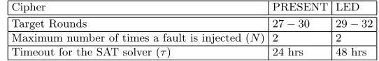
Table 2: Setup for the ML on PRESENT and LED
Cipher PRESENT LED
Target Rounds 27−30 29−32
Maximum number of times a fault is injected (N) 2 2
0 20 40 60 80 100 120 Features No 0.00 0.02 0.04 0.06 0.08 0.10 0.12 0.14 0.16 Fe atu res Im po rta nc e PRESENT (a)
50 100 150 200 250 300 350 400 450 500 550 No of training data 0.5 0.6 0.7 0.8 0.9 A cc ur ac y (b)
0.0 0.2 0.4 0.6 0.8 1.0
False Positive Rate (FPR)
0.0 0.2 0.4 0.6 0.8 1.0 Tr ue Po si ti ve R at e (T PR )
ROC - PRESENT
(c)
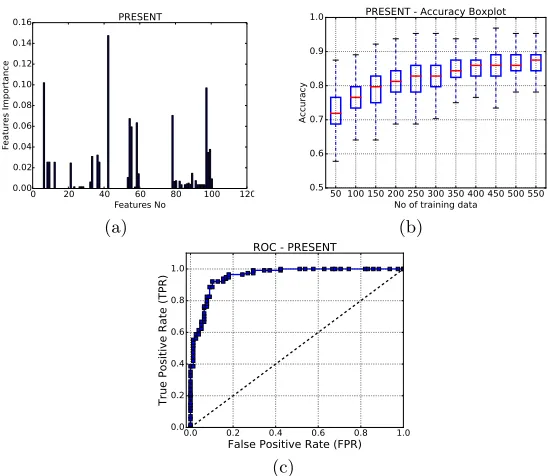
Fig. 3: Machine learning results for PRESENT. (a) Feature importance; (b) ROC curve; and (b) Variation of accuracy with the size of training set.
The basics of PRESENT block cipher has already been described in Sec. 3.2. Several fault attack examples have been proposed on PRESENT, mostly tar-geting the 29-th and 28-th round of the cipher as well as the key schedule of PRESENT [10, 21, 34–37]. Zhang et.al. [10] presented an AFA on PRESENT, requiring 2 bit-fault instances on average, at the 28-th round of the cipher in the best case. The solving times of the corresponding CNFs are mostly around 3 minutes.
Experimental Setup In order to validate the proposed framework, we create
(N) was restricted to 2, (that is,N can assume values 1 and 2) considering low fault-complexities of DFAs. Interestingly, it was observed that the nibble fault instances (injected 2 times in succession) at 28-th round do not result in suc-cessful attacks, even after 2 days. Further, many of these instances (almost 12%) take 16−24 hrs of solving time. No, successful attack instances were found taking time beyond 24 hours in our experiments, which were conducted on a machine with Intel Core i5 running CryptominiSAT-5 [33] as the SAT solver in a single threaded manner. We thus set the SAT timeoutτ= 24 hours for PRESENT. For the sake of experimentation, we exhaustively characterized a set of 1000 samples from the fault space of PRESENT and LED, individually. However, one should note that such exhaustive characterization was only required to prove the appli-cability of the proposed methodology, and in practice, a much smaller number of instances are required for training the ML classifier, as well shall show later. For every new cipher, suchprofiling should be performed only once just to build the ML classifier.
Feature Selection The first step in our experiments is to evaluate the feature
set. Although we started with a well-accepted feature set, it is always interesting to know how these features impact the learning process and which are the most important features in the present context. Identification of the main contributing features for a given problem may also lead to significant reduction of the feature space dimensionality by the selection of actually useful features, which also re-duces the chances of overfitting. We therefore perform a quantitative assessment of the importance of various features using the RF algorithm. Before proceed-ing further, it is worth mentionproceed-ing that some of the SATzilla features might be computationally expensive depending on problem instances. It was found that the unit propagation features (which belong to the group of DPLL probing fea-tures) and the linear programming features in our case takes even more than 15 minutes of computing time for certain instances. As a result, we did not consider them in our experiments which left us with 123 features in total.
In this work, we evaluate the feature importance based on themean decrease of gini-impurityof each feature during the construction of the decision trees [38]. Every nodeζ, in a given decision treeγ, of an RF Γ imposes a partition on the dataset by putting some threshold condition on a single feature, so that similar samples end up in the same partition. The optimal split at a node is calculated based on a statistical measure which quantifies how well a potential split is separating the samples of different classes at this particular node. The
gini-impurity is one of the most popular measure for such purposes and is actually
used in random forests [38]. Let us assume that a nodeζ in some decision tree
γ∈Γ has total|ζ|samples among which the subsetζq consists of samples from
classq∈ {0,1}. Then thegini-impurity ofζis calculated as:
feature θ, and the gini-impurity of these two nodes are G(ζlef t) and G(ζright),
respectively. Then the decrease in impurity at the node ζ, due to this specific split is calculated as:
∆G(ζ) =G(ζ)−plef tG(ζlef t)−prightG(ζright) (11)
where, plef t= | ζlef t|
|ζ| , andpright= | ζright|
|ζ| . In an exhaustive search over all
vari-ablesθ available atζ and the space of correspondingtθs, the optimal split atζ,
for a particular treeγcan be determined which is quantified as ∆θG(ζ, γ). In the
calculation of feature importance, decrease in gini-impurities are accumulated in a per-variable basis and the importance value of the feature θ, is calculated as follows:
IG(θ) =
X
γ∈Γ
X
ζ∈γ
∆θG(ζ, γ) (12)
The result of the feature importance assessment experiment is presented in Figure 3a, where the X-axis represents the index of a feature and the Y-axis represents its importance scaled within an interval of [0,1]. It is interesting to observe that, there are almost 66 features, for which the importance value is 0. Further investigation reveals that these features obtain constant values for all the instances. As a result, they can be safely ignored for the further experiments. It can be observed from Figure 3a, that the feature no. 42 is the most impor-tant one for our experiments. This feature corresponds to the aggregated com-putation time for the Variable-Clause Graph (VCG) and Variable-Graph (VG) graph-based features. A VCG is a bipartite graph, with nodes corresponding to each variable and clause. The edges in this graph represent the occurrence of a variable in a clause. The VG has a node for each variable and an edge between variables that occur together in at least one clause. Intuitively, the computation time is a crude representative for the dense-nature of these graphs, which is usu-ally high if the search space is very large and complex. However, it is difficult to directly relate this feature with quick solvability of an instance as other selected features also play a significant role. In fact, it was observed that every structural feature group have some contribution in the classification, which is somewhat expected (feature no. 0−59 in Figure 3a). In contrast, the contributions from the runtime features were not so regular. In particular, only the survey propagation features (based on estimates of variable bias in a SAT formula obtained using probabilistic inference [30].) were found to play some role in the classification (feature no. 79-96 in Figure 3a). Interestingly, the features 98−100, which corre-sponds to the approximate search-space size (estimated with the average depth of contradictions in DPLL search trees [31]), were found to play some role in the classification. This is indeed expected, as the classification margin in this work is defined based on the search space size.
Classification We next measured the classification accuracy of the RF
Table 3: Misclassification Handling for PRESENT SValue 0.10 0.12 0.14 0.16 0.18 0.20 0.22 0.24 0.26 0.28 0.30 % Sensitive Instances 6.0 6.0 10.0 13.2 17.2 20.4 20.4 22.0 22.8 24.8 27.6 % False Negatives beyondS 4.1 4.1 3.0 1.8 0.6 0.2 0.0 0.0 0.0 0.0 0.0
training and validation sets were chosen from a set of 640 labeled samples (the remaining 360 samples collected at the profiling phase were utilized for further validation and false negative removal experiments), where the sizes of them are in the ratio 7 : 3. The sample set consists of 320 exploitable and 320 unexploitable fault instances in order to achieve an unbiased training. The average accuracy obtained in our experiment was 85%. We also provide the Receiver Operating Characteristics (ROC) curve for the RF classifier, which is considered to be a good representative for the quality of a classifier. The Area Under Curve (AUC) represents the goodness of a classifier, which ranges between 0 to 1 with higher values representing a better classifier. The ROC curve for the PRESENT exam-ple is provided in Fig. 3c, which shows that the classifier performs reasonably well in this case. Fig. 3b presents the variation of accuracy with the size of train-ing dataset as a box plot. It can be observed that reasonable accuracy can be reached within 450 training instances (which is around 70% of our dataset size) and accuracy does not improve much after that.
Handling False Negatives Although our classifier reaches a reasonable good
accuracy of 85%, there are almost 15% instances which get misclassified in this process, which contains both false positives and false negatives. As pointed out in Sec. 4.5, false negatives are not acceptable in certain scenarios. The approach presented in Sec. 4.5 critically depends on the threshold parameter S, which must be set in a way so that the percentage of false negatives become 0 or at least negligibly small. If the percentage of instances below S is too high, it would be costly to estimate all of them via exhaustive SAT solving. However, the reasonably good accuracy of our classifier suggests that the percentage of such sensitive instances may not be very high. We tested our proposed fix from Section. 4.5 on a new set of 250 test instances with different S values. Table 3 presents the outcome of the experiment. The percentage of instances to be justi-fied via SAT solving and the percentage of false negatives beyondSis presented in the table for each choice ofS. It can be observed from Table 3 that a thresh-old of 0.22 nullifies the number of false negatives and keeps the percentage of sensitive instances (see Section. 4.5) to 20%, which is indeed reasonable.
Gain over Exhaustive SAT Solving It would be interesting to estimate the
reasonable-sized sample of 10000 fault instances, the exhaustive characterization with SAT solving only would be impractical. Considering a timeout threshold of 24 hrs (τ= 24 hrs), characterization of these many instances even with a parallel machine with a reasonable number of cores would take an impractical amount of time. For example, if one considers a 24 core system, the characterization would require 416 days, in the worst case. Even with an optimistic consider-ation of roughly 50% of the instances hitting the timeout threshold, the time requirement is still high. In contrast, the proposed framework can provide a fairly reasonable solution. Firstly, the size of the training set is extremely small, and also saturates after reaching a reasonable accuracy. One can rapidly characterize any number of fault instances after training with a reasonable error probability and the time requirement for that is insignificant. For a statistical understand-ing of the exploitable fault space, such error bounds can be reasonably tolerated. For even more security-critical applications, like evaluating a countermeasure or quantification of security bounds, the misclassified attack instances can be cru-cial. The proposed method works fine even in those cases with a reasonable overhead of characterizing 22% of the instances exhaustively. For a set of 10000 fault instances, it would require 83 days, even in the worst case which is much better than the figures obtained with exhaustive characterization.
Discussion One of the goals of the ML framework is to discover new attacks
while trained on a set of known attack instances. It was found that the proposed framework is able to do that with reasonably high accuracy. More specifically, we found that if the training set contains only of fault instances injected at even-numbered nibbles at the 28th round, it can successfully predict all attacks from odd-numbered nibbles. This clearly indicates the capability of discovering new attacks. The proposed framework also successfully validated the claim that with the bit permutation based linear layer of PRESENT, the fault diffusion (and thus the attack) strongly depends on the plaintext and the value of the injected fault. Although this might not be a totally new observation, our framework figures it out, automatically, and can quantify this claim statistically within reasonable amount of time.
5.2 Exploitable Fault Space Characterization for LED
50 100 150 200 250 300 350 400 450 500 550 No of training data 0.5
0.6 0.7 0.8 0.9 1.0 1.1 1.2
A
cc
ur
ac
y
LED - Accuracy Boxplot
(a)
0.0 0.2 0.4 0.6 0.8 1.0
False Positive Rate (FPR)
0.0 0.2 0.4 0.6 0.8 1.0
Tr
ue
Po
si
ti
ve
R
at
e
(T
PR
)
(b)
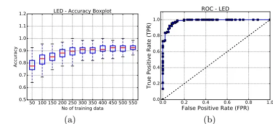
Fig. 4: Machine learning results for LED. (a) ROC Curve; and (b) Variation of accuracy with the size of training set.
the cipher which requires 43 nibble faults to be injected at a particular nibble. Jovanovic et. al. [7] and Zhao et. al. [9] independently presented AFA attacks on LED, where they show that it is possible to attack the cipher at 30th round with a single fault instance.
ML Experiments In this work, we mainly focus on the last 5 rounds of the
LED cipher. However, unlike the previous experiment on PRESENT, a slightly different strategy was adopted. In order to examine the proper potential of the ML model in discovering newer attack instances across different rounds, we in-tentionally trained it with samples from the 30 and the 31st rounds and tested it on instances from rounds 29 and 32. The RF model is trained with a total of 450 instances from the 30 and the 31st rounds and tested on 190 instances from rounds 29 and 32. The setup for the data acquisition is given in Table 2. The ac-curacy box plot and ROC curve for the classifier are provided in Fig. 4a and 4b, respectively. It can be observed that the accuracy is almost 93%. The features used were similar to the PRESENT experiments. Handling of misclassification was also performed and the result is presented in Table. 4.
Discovery of New Attacks We observed a quite interesting phenomenon
in this experiment which clearly establishes the capability of the ML tool in discovering newer attack instances. More specifically, we found that the ML tool can identify attacks on 29th round of the cipher, even if it not trained with any instances from the 29th round. The attack instances observed at the 29th round of LED are mainly bit-fault instances with 2 fault injections. Attacks
on the 29th round of LED are usually difficult than the 30th round
attacks [41, 42], and it is quite remarkable that the ML model can figure out difficult attacks just by learning easier attack instances.
Discussion So far we have discussed two ciphers with same S-Box and different
example, almost all of the 30 round nibble faults in LED resulted in a successful attack, whereas for PRESENT there was a significant number of unexploitable instances at 28th round. Form the perspective of an adversary, targeting a ci-pher having bit-permutation based diffusion layers thus become a little more challenging as he/she must attack it with more number of fault injections in order to obtain a successful attack.
5.3 Analyzing the Effect of S-Boxes on Fault Attacks
Table 4: Misclassification Handling for LED
SValue 0.10 0.12 0.14 0.16 0.18 0.20 0.22 0.24 0.26 0.28 0.30 % Sensitive Instances 4.2 6.0 6.0 11.6 13.2 15.2 17.6 17.6 21.2 23.8 23.8 % False Negatives beyondS 2.4 1.6 0.9 0.3 0.18 0.0 0.0 0.0 0.0 0.0 0.0
Table 5: Mathematical Properties of PRESENT, SERPENT, and SKINNY S-Boxes
Property PRESENT SERPENT SKINNY
Size 4×4 4×4 4×4
Differential Branch Number 3 3 2
Differential Uniformity 4 4 4
Max. Degree of Component Functions 3 3 3 Min. Degree of Component Functions 2 2 2
Linearity 8 8 8
Nonlinearity 4 4 4
Max. Differential Probability 0.25 0.25 0.25 Max. Degree of Polynomial Representation
(with Lexicographic Variable Ordering) 3 3 3
The S-Boxes are one of the most important resources in a block cipher con-struction. However, till date, no quantitative analysis was performed to evaluate the effect of S-Boxes on the fault attacks as such. In classical DFA, the attack complexity is related with the average number of solutions of the S-Box differ-ence equations having the form S(x)⊕S(x⊕α) = β. However, S-Boxes were never characterized in the context of fault attacks considering the cipher as a whole. The characterization of the exploitable fault space in this work gives us the opportunity to perform such analysis.
0 2 4 6 8 10 12 14 16 Nibbles 0.0 0.2 0.4 0.6 0.8 1.0 Pe rc en ta ge ( % ) PRESENT exploitable not-exploitable (a)
0 2 4 6 8 10 12 14 16
Nibbles 0.0 0.2 0.4 0.6 0.8 1.0 Pe rc en ta ge ( % ) SERPENT exploitable not-exploitable (b)
0 2 4 6 8 10 12 14 16
Nibbles 0.0 0.2 0.4 0.6 0.8 1.0 Pe rc en ta ge ( % ) SKINNY exploitable not-exploitable (c)
Fig. 5: Exploitable Fault Spaces with. (a) PRESENT Box; (b) SERPENT S-Box; and, (c) SKINNY S-Box.
ML-based framework. For the sake of simplicity, we only tested with nibble faults injected with N = 2 (that is two times for each fault instances) at the 28th round. The obtained test accuracies were similar to that of the PRESENT experiment and so we do not repeat them here. Further, for each of the S-Box case, we consider 1000 fault instances for each nibble location (there are total 16 nibble locations.). The characterized fault spaces of the three S-Box test cases are depicted in Fig. 5a, 5b and 5c , respectively. It is interesting to observe that although the PRESENT and SERPENT S-Box results in almost similar behavior, the SKINNY S-Box results in a significantly different fault distribu-tion. More specifically, whereas most of the fault instances for the PRESENT
SB
SB SB SB SB SB
SB SB SB SB
SB
SB SB SB SB SB
SB SB SB SB
(a) (b)
(c) (d)
SB SB SB SB SB SB SB SB SB SB SB SB SB SB SB SB
SB SB SB SB SB SB SB SB SB SB SB SB SB SB SB SB SB 28 29 30 (e) round (i-1) round i round (i-1) round i round (i-1) round i round i round (i-1)
and SERPENT are exploitable (60% exploitable faults on average), the situation is reverse in the case of SKINNY (23% exploitable faults on average).
Analysis of the Observations In order to explain the observations made in
this experiment, we had an in-depth look in the 3 S-Boxes as well as the diffusion layer of PRESENT. The fault diffusion in PRESENT linear layer depends on the number of active S-Boxes (S-Boxes whose inputs are affected by the faults.).For a multi-round fault propagation, the number of active S-Boxes in theith round
depends on the Hamming Weights (HW) of the output S-Box differential in the
(i−1)thround.Fig. 6 emphasizes this claim with a very simple example. The lines
colored red indicate non-zero differential value and the red S-Boxes are the active S-Boxes. Now let us consider the fault diffusion tree for the 28th round nibble fault injection in the PRESENT structure, shown in Fig. 6e up to 30th round, for convenience. It can be observed that most of the S-Boxes obtain an input difference of 1 bit. In other words, the inputs of the S-Boxes will have a single bit flipped. With this observation, the investigation boils down to the following question –If the HW of the input difference of an S-Box is1, what is the HW of
the output difference? For all three S-Boxes considered, the average HW of the
output difference should be 2 when the average is considered over all possible input differences (this is due to the Strict Avalanche Criteria (SAC)). However, for the typical case, where the HW of the input difference is restricted to 1, the average HW of the output differences vary significantly. More specifically, the average is quite low for the SKINNY S-Box where it attains a value of 2.2. For the PRESENT S-Box, the value is 2.45 and for SERPENT it is 2.5. This stems from the fact that, for the SKINNY S-Box, there exists input difference values,
for which the HW of the output differences become 1. Whereas for PRESENT
and SERPENT S-Boxes, the minimum HW of the output differences is 2 for
any given input difference. In essence, the fault diffusion with PRESENT and
SERPENT S-Box is more rapid on average, than the SKINNY S-Box, which got reflected in the profile observed for exploitable fault spaces.
The result presented in this subsection is unique from several aspects. Firstly, it shows empirically that even if the S-Boxes are mathematically equivalent, they may have different effects in the context of fault attacks. Secondly, the proposed framework of ours can identify such interesting phenomenon for different cipher sub-blocks, which are otherwise not exposed from standard characterization. This clearly establishes the efficacy of the proposed approach.
6
Conclusion
framework proposed here is not limited to block ciphers only. It is quite well-known that even stream ciphers, public key algorithms [44] and hash functions can be mapped to algebraic systems [45]. From that perspective, the framework can be easily extended to handle those cases.
In this paper, we have elaborated an application of exploitable fault char-acterization for the evaluation of cipher sub-operations in the context of fault attacks. However, several other applications are possible as already anticipated in the introduction section. One of the potential applications could be the guided synthesis of countermeasures for resource-constrained environments. Through a statistical characterization of the exploitable fault space in a per-round man-ner, one can potentially identify locations which are the most sensitive to the fault attacks. One can then implement costly countermeasures for those posi-tions only, whereas less sophisticated countermeasures would work well for the rest of the cipher. Another important application scenario could be the testing of implementations and countermeasures with a large number of exploitable fault instances, rather than with random faults. Such testings are highly desired to correctly evaluate fault attack threats, or to certify a system against such attacks and can be realized quite efficiently with the proposed framework.
References
1. V. Rijmen and J. Daemen, “Advanced encryption standard,” in Proc. of FIPS Publications, NIST, pp. 19–22, 2001.
2. M. Tunstall, et. al., “Differential fault analysis of the advanced encryption standard using a single fault,” in WISTP. Springer, 2011, pp. 224–233.
3. E. Biham, et. al., “SERPENT: A new block cipher proposal,” inFSE. Springer, 1998, pp. 222–238.
4. A. Bogdanov, et. al., “PRESENT: An ultra-lightweight block cipher,” in CHES. Springer, 2007, pp. 450–466.
5. J. Guo, et. al., “The LED Block Cipher,” inCHES. Berlin, Heidelberg: Springer Berlin Heidelberg, 2011, pp. 326–341.
6. N. T. Courtois, et. al., “Fault-algebraic attacks on inner rounds of DES,” e-Smart’10 Proceedings: The Future of Digital Security Technologies, 2010.
7. P. Jovanovic, et. al., “An algebraic fault attack on the LED block cipher.”IACR Cryptology ePrint Archive, vol. 2012, p. 400, 2012.
8. F. Zhang, et. al., “Improved algebraic fault analysis: A case study on PICCOLO and applications to other lightweight block ciphers,” inCOSADE. Springer, 2013, pp. 62–79.
9. X. Zhao, et. al., “Algebraic differential fault attacks on LED using a single fault injection.”IACR Cryptology ePrint Archive, vol. 2012, p. 347, 2012.
10. F. Zhang, et. al., “A framework for the analysis and evaluation of algebraic fault attacks on lightweight block ciphers,”IEEE Trans. Inf. Forensics Security, vol. 11, no. 5, pp. 1039–1054, 2016.
11. P. Khanna, et. al., “XFC: A Framework for eXploitable Fault Characterization in Block Ciphers,” inDAC. IEEE, 2017.
13. D. Boneh, et. al., “On the importance of checking cryptographic protocols for faults,” inEUROCRYPT. Springer, 1997, pp. 37–51.
14. E. Biham and A. Shamir, “Differential fault analysis of secret key cryptosystems,” CRYPTO, pp. 513–525, 1997.
15. G. Piret and J.-J. Quisquater, “A differential fault attack technique against SPN structures, with application to the AES and KHAZAD,” in CHES, vol. 2779. Springer, 2003, pp. 77–88.
16. C. Giraud, “DFA on AES,” in Int. Conf. Adv. Encryption Standard. Springer, 2004, pp. 27–41.
17. S. S. Ali and D. Mukhopadhyay, “A differential fault analysis on AES key schedule using single fault,” inFDTC. IEEE, 2011, pp. 35–42.
18. T. Fuhr, et. al., “Fault attacks on AES with faulty ciphertexts only,” in FDTC. IEEE, 2013, pp. 108–118.
19. B. Robisson and P. Manet, “Differential behavioral analysis,” inCHES. Springer, 2007, pp. 413–426.
20. N. F. Ghalaty, et. al., “Differential fault intensity analysis,” in FDTC. IEEE, 2014, pp. 49–58.
21. N. F. Ghalaty, et. al., “Differential fault intensity analysis on PRESENT and LED block ciphers,” inCOSADE. Springer, 2015, pp. 174–188.
22. J. Bl¨omer and J.-P. Seifert, “Fault based cryptanalysis of the advanced encryption standard (AES),” inCAV. Springer, 2003, pp. 162–181.
23. N. T. Courtois and J. Pieprzyk, “Cryptanalysis of block ciphers with overdefined systems of equations,” inASIACRYPT. Springer, 2002, pp. 267–287.
24. D. Mitchell, et. al., “Hard and easy distributions of SAT problems,” in AAAI, vol. 92, 1992, pp. 459–465.
25. F. Hutter, et. al., “Performance prediction and automated tuning of randomized and parametric algorithms,”CP, vol. 4204, pp. 213–228, 2006.
26. E. Nudelman et. al., “Understanding random SAT: Beyond the clauses-to-variables ratio,” inCP. Springer, 2004, pp. 438–452.
27. F. Hutter, et. al., “Algorithm runtime prediction: Methods & evaluation,”Artificial Intelligence, vol. 206, pp. 79–111, 2014.
28. L. Xu, et. al., “SATzilla: portfolio-based algorithm selection for SAT,”Journal of AI research, vol. 32, pp. 565–606, 2008.
29. K. Leyton-Brown, et. al., “Empirical hardness models: Methodology and a case study on combinatorial auctions,”J. ACM, vol. 56, no. 4, p. 22, 2009.
30. E. Hsu, et. al., “Probabilistically estimating backbones and variable bias: Experi-mental overview,” inCP. Springer, 2008, pp. 613–617.
31. L. Lobjois,et al., “Branch and bound algorithm selection by performance predic-tion,” inAAAI/IAAI, 1998, pp. 353–358.
32. K. Varshney, et. al., “A risk bound for ensemble classification with a reject option,” inSSP IEEE, 2011, pp. 769–772.
33. M. Soos, et. al, “Extending SAT solvers to cryptographic problems,” in SAT. Springer, 2009, pp. 244–257.
34. G. Wang and S. Wang, “Differential fault analysis on PRESENT key schedule,” in CIS. IEEE, 2010, pp. 362–366.
35. X. Zhao, et. al., “Fault-propagate pattern based DFA on PRESENT and PRINT-cipher,”J. Wuhan Univ. Natur. Sci., vol. 17, no. 6, pp. 485–493, 2012.
36. N. Bagheri, et. al., “New differential fault analysis on PRESENT,” EURASIP J Adv Signal Process., vol. 2013, no. 1, p. 145, 2013.
38. L. Breiman, “Random Forests,”Machine Learning, vol. 45, no. 1, pp. 5–32, 2001. 39. W. Li, et. al., “Single byte differential fault analysis on the LED lightweight cipher in the wireless sensor network,”Int. J. Comput Int Sys., vol. 5, no. 5, pp. 896–904, 2012.
40. P. Jovanovic, et. al., “A Fault Attack on the LED Block Cipher.” in COSADE. Springer, 2012, pp. 120–134.
41. W. Li, et. al., “Impossible differential fault analysis on the led lightweight cryp-tosystem in the vehicular ad-hoc networks,”IEEE Trans. IEEE Trans Dependable Secure Comput., vol. 13, no. 1, pp. 84–92, 2016.
42. G. Zhao, et. al., “Differential fault analysis on LED using Super-Sbox,” IET In-formation Security, vol. 9, no. 4, pp. 209–218, 2014.
43. C. Beierle, et. al., “The SKINNY family of block ciphers and its low-latency variant MANTIS,” inCRYPTO. Springer, 2016, pp. 123–153.
44. J. Faugere, et. al., “Algebraic Cryptanalysis of Hidden Field Equation (HFE) Cryp-tosystems Using Gr¨obner Bases.,” inCRYPTO. Springer, 2003, pp. 44–60. 45. P. Luo, et. al., “Algebraic fault analysis of SHA-3,” inDATE. IEEE, 2017, pp.