Vibration Analysis using 3D Image Correlation Technique
T.Siebert1a, K. Splitthof1
1Dantec Dynamics GmbH, Kaessbohrerstr. 18, D-89077 Ulm, Germany
Abstract.. Digital speckle correlation techniques have already been successfully proven to be an accurate displacement analysis tool for a wide range of applications. With the use of two cameras, three dimensional measurements of contours and displacements can be carried out. With a simple setup it opens a wide range of applications. Rapid new developments in the field of digital imaging and computer technology opens further applications for these measurement methods to high speed deformation and strain analysis, e.g. in the fields of material testing, fracture mechanics, advanced materials and component testing. The high resolution of the deformation measurements in space and time opens a wide range of applications for vibration analysis of objects. Since the system determines the absolute position and displacements of the object in space, it is capable of measuring high amplitudes and even objects with rigid body movements. The absolute resolution depends on the field of view and is scalable. Calibration of the optical setup is a crucial point which will be discussed in detail. Examples of the analysis of harmonic vibration and transient events from material research and industrial applications are presented. The results show typical features of the system.
1 Introduction
In recent years optical full-field measuring techniques are increasingly being used in research and industry as development and design tools for improved characterization of materials and components. Besides moiré and interferometer based techniques the digital image correlation method is widely used for full-field and three dimensional displacement measurements [1-4].
Digital Image Correlation (DIC) is a full-field image analysis method, based on grey value digital images, that allows determination of the contour and surface displacements of an object under load in three dimensions. Due to rapid new developments of high resolution digital cameras and computer technology, the applications for these measurement methods have broadened. Since the system determines the absolute position and displacement of the object in space, deformation measurements with very high resolution are possible even under the presence of large deformation amplitudes and macroscopic rigid body movements.
The displacement resolution depends on the field of view (typically down to 10-5 of the field of view) and therefore is scalable, e.g. a few µm for an A4 paper size field of view depending on the
a e-mail : [email protected] © Owned by the authors, published by EDP Sciences, 2010 DOI:10.1051/epjconf/20100611004
number of pixels used. The measurable displacement range for this configuration is from µm up to several cm.
Out of the contour and displacement measurement, the image correlation technique provides material parameters far into the range of plastic deformation. Further data analysis tools allow the determination of the location and the amplitude of the maximum strain, the global strain distribution and behaviour of crack growth, which are important parameters for material testing and fracture mechanics. Analyzing the temporal displacement by using e.g. Fourier analysis can give information about modal shape and vibration amplitudes.
2 Principles of Digital Image Correlation
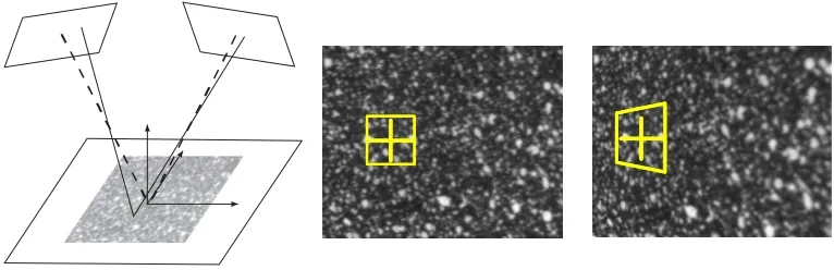
Two imaging sensors, looking from different positions at an object, similar to human vision, provide enough information to perceive the object as three dimensional. Using a stereoscopic camera setup (figure 1, left), each object point is focused on a specific pixel in the image plane of the respective camera.
With the knowledge of the imaging parameters for each camera (intrinsic parameters: focal length, principle point and distortion parameters) and the orientations of the two cameras with respect to each other (extrinsic parameters: rotation matrix and translation vector), the position of each object point in three dimensions can be calculated.
Fig. 1. Principle of stereoscopic setup (left) and grey value pattern in different images on the camera.
Using a stochastic intensity pattern on the object’s surface, the position of each surface point in the two images can be identified by applying a correlation algorithm. By using this correlation algorithm, a matching accuracy of the original and the transformed facet of better than 0.01 pixel can be achieved [5].
The stochastic pattern can be applied easily with a colored spray paint, printing or other transfer methods. The size and distribution does influence the achievable resolution. An investigation about an optimum pattern and evaluation parameters can be found e.g. at Lecompte et al [6].
2.1 Calibration
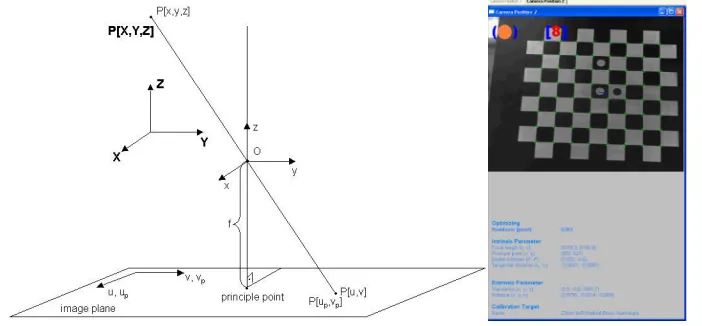
The quality of the measurement is ensured by the exact knowledge of the intrinsic and extrinsic imaging parameters of the system. The imaging model is based on a pinhole model (figure 2). Thus the projection of the object point on the CCD is defined by the intersection of the line from the object point through the principle point of the imaging system and the CCD. The distance of the principle point to the image plane is the focal length f, the projection on the image plane the position of the optical axis on the CCD.
14th International Conference on Experimental Mechanics
The calibration process is integrated in the measurement software. During the calibration process the calibration points, which might be dots or intersection of lines, are detected automatically and displayed online on screen. Both cameras capture the images of the calibration target at the same time, the calibration parameters from both cameras will be calculated.
Typically eight images are sufficient to calculate all calibration parameters accurately. An online procedure and the direct user feedback allow an easy, reliable and fast calibration of the system.
Fig. 2. Pin-hole camera model (left) and calibration target and calculated calibration parameters (right).
2.2 Acquisition
Depending on the type of camera which is used for the image acquisition, several parameters and adjustments of the cameras can be made, e.g. exposure time, frame rate, brightness, contrast and area of interest. Typically a series of a few up to several hundreds of images are acquired and saved during the experiment. The acquisition can be started manually or fully automatically using various types of triggering. These images, combined with the calibration parameters, are the base for the evaluation.
2.3 Evaluation
By applying the correlation algorithm, the position of all object points can be identified in the image from both cameras. Using the intrinsic and extrinsic parameters of the system, the 3-dimensional coordinates for each object point can be calculated leading to a 3-dimensional contour of the object. Following the changes of the grey value pattern for each camera along the loading steps, the surface displacements of the object are calculated. The matching accuracy of the correlation algorithm resulting in a displacement resolution down to 1/100 000 of the field of view for a MegaPixel CCD camera. For an A4 paper size this gives a resolution in displacement of down to 3-4 µm. [5-8].
3 Applications
In the following we present three dynamic applications: a vibration analysis of a membrane, a shock excitation of an aluminium plate and an excitation of a circuit board using white noise.
3.1 Vibration of a membrane
During this experiment the vibration of a rubber membrane in front of a loudspeaker, which is excited close to a resonance frequency, was investigated. The size of the evaluated area is about 300x260mm2. The used rubber material has a porous surface, which gives a statistical grey value
distribution, thus no extra preparation of the surface was necessary. A white colour was used to increase the amount of diffusely reflected light. The loudspeaker was excited at 59.9 Hz where a membrane was vibrating in resonance.
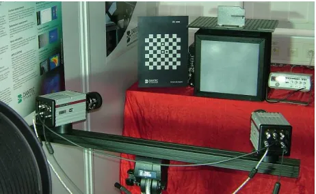
For image acquisition, high-speed cameras (Nanosense MK III) with 1280 x 1024 pixels resolution where used. The maximum frame rate at full resolution of these cameras is 1000Hz, for this measurement the frame rate was reduced to 625Hz. In figure 3 the setup including the high-speed cameras and the loudspeaker, is shown.
Fig. 3. Experimental setup with high-speed cameras, calibration target, loudspeaker and frequency generator for vibration measurement.
The image acquisition was started previous to the excitation of the loudspeaker. For the evaluation 150 images corresponding to 0.25 seconds of testing were processed.
The results of the measurement are displayed as a 3-dimensional model. On the surface of the object’s model different data can be mapped in order to display the full field information. The different data are contour information (e.g. distances to Best-Fit plane), displacements (e.g. absolute X-, Y- or Z-deformation) or strains (e.g. principal strains). Figure 5 shows the full field display of the out of plane deformation of the membrane at the maximum elongation during the vibration. The colours represent the amplitudes of displacements. In the lower part of the graphic a spatial profile along the horizontal direction is displayed.
14th International Conference on Experimental Mechanics
Fig. 4. Full field out-of-plane deformation of the membrane at maximum deflection of the centre (top left and top right). Spatial profile along a horizontal line (bottom left) and temporal plot of the
displacement of the centre point (bottom right).
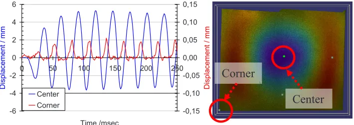
For the next measurement the frequency of excitation was set to another resonance at 36.5 Hz. Figure 5 shows the amplitude of vibration of the centre point and of a point in the lower left corner. The point in the centre vibrates with amplitude of about 5 mm symmetrically in the positive and negative direction. At the corner point the membrane is fixed on the housing of the loudspeaker, thus this point moves only in the positive direction. The amplitude is just about 0.05 mm. This example demonstrates the dynamic range, which can be covered with a single full field measurement.
-6 -4 -2 0 2 4 6
0 50 100 150 200 250
Time /msec
D
isp
la
ce
men
t / mm
-0,15 -0,10 -0,05 0,00 0,05 0,10 0,15
D
isp
la
ce
men
t / mm
Center Corner
Fig. 5. Out-of plane displacement of points in the centre and in the corner over time.
3.2 Shock excitation
Besides harmonic events the technique of image correlation is suitable to analyze transient events. For the measurement which is presented here, an explosive charge was used for excitation, which was positioned behind the backside of a square shaped aluminium plate with a size of 70 x 70 cm2.
The first measurement was performed with an image acquisition rate of 1 kHz, for a second measurement the frame rate was increased to 5 kHz. With both measurements the full field behaviour of the plate could be analyzed.
The series of images from this event can be processed like the images from the harmonic vibration before. As an example figure 6 shows the evolution of the displacement of the plate up to 5 msec after firing of the explosive charge. For a better understanding the displacements are scaled by a factor of 300.
Center
Fig. 6. Full field displacement (scaled by a factor of 300) of the plate.
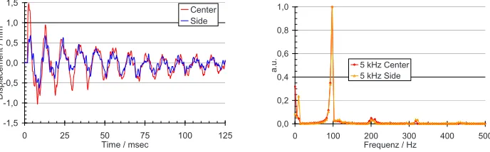
From this full field information single points can be selected, analyzing their temporal evolution. The displacements of the centre point and a point close to the border over a period of 125 msec are plotted in figure 7. The maximum amplitude of the centre is about 1.5 mm; it is about 0.5 mm of the point near the border. Due to the strong damping the amplitude decreases quickly down to 0.3 mm after 100 msec. Because of the presence of higher frequencies of vibration, which were stimulated by the shock excitation as well, the temporal displacement curves are not completely smooth.
-1,5 -1,0 -0,5 0,0 0,5 1,0 1,5
0 25 50 75 100 125 Time / msec
D
ispl
a
ce
ment / mm
Center Side
0,0 0,2 0,4 0,6 0,8 1,0
0 100 200 300 400 500
Frequenz / Hz
a.
u. 5 kHz Center
5 kHz Side
Fig. 7. Out-of plane displacement of two points up to 125 msec after firing the explosive charge (left) and the spectrum (right).
A Fourier Transformation from these temporal displacements clearly reveals these vibration frequencies. Figure 8 shows the main frequencies for the point in the centre and a point close to the border. The main frequency for both points is not very sharp and is between 92 and 97 Hz. The amplitudes of the higher frequencies are much smaller also with a broad bandwidth.
Using the time evolution of the displacement of individual points out of the full field data, the different frequencies of vibration, which were excited with the shock event, were clearly resolved. Since the data of all object points are recorded simultaneously (no scanning is required), this method could be advantageously used for the study of transient events. The mode shape of the vibration could easily be analyzed.
3.3 Noise excitation
A circuit board was mounted on a shaker in a horizontal position. In an area of about 65 x 30 mm the movement of the circuit board was recorded at 2 kHz frame rate. The shaker was driven using white noise in a frequency range between 200 and 1 kHz. In Fig. 8 the image of one camera is showing the area under investigation and the full-field result as well as the displacement of a single point over time. The displacement of the point is in the range of ca. 40 µm.
14th International Conference on Experimental Mechanics
Fig. 8. Field of view (left), full-field displacement at one measurement step (right top) and displacement of marked point (cross) over measurement steps (right bottom).
By applying a frequency analysis at different points the main frequencies of the object can be determined. In this case an accelerometer indicates a main frequency at about 770 Hz. This frequency was found mainly in the centre of the board where the accelerometer was placed and no elements are located. The reconstruction of the mode shape at this frequency is shown in Fig. 9. The amplitude is in the range of 10 µm with a smooth shape which does not show areas of critical stressing of the board.
-40 -20
0 20
40 -30 -20
-10 0 10 20 -0.01 0 0.01 0.02
y-coordinate / mm x-coordinate / mm
A m plit ude / m m -0.01 -0.005 0 0.005 0.01 0.015 0.02
Fig. 9. Reconstructed mode shape at 770 Hz.
A frequency analysis at a point close to the longitudinal connector showed another peak at about 535 Hz. The reconstructed mode shape is shown in Fig. 10. The amplitude of about 20 µm doubles the amplitude at 770 Hz. The shape of this mode generates also gradients of displacement and strain in an area of the connector and small electronic elements on the board. This frequency at 535 Hz will lead to higher chance of failure than other frequencies.
The application of this full-field method in combination with a frequency analysis allows the identification and reconstruction of the different mode shapes. This gives quantitative information about the behaviour and damage of the sample at different frequencies.
-40 -20
0 20
40 -30 -20
-10 0 10 20 -0.01 0 0.01 0.02
y-coordinate / mm x-coordinate / mm
A m pli tude / m m -0.01 -0.005 0 0.005 0.01 0.015 0.02
4 Conclusion
This paper shows recent developments and applications of digital image correlation. Improvements in the calibration procedure significantly ease the handling of the system, while decreasing calibration time and enhancing the reliability of the results. Due to the modular concept of the hardware and the software this system can be used for a wide range of applications. Based on a full field method, this technique allows the determination of displacement amplitudes and vibration phases with high spatial and temporal resolution and within a large dynamic range. Amplitudes from m to µm and frequencies up to several tens of kHz could be covered, giving rise to applications of dynamic displacement and dynamic strain measurements. The use of high speed cameras offers the chance of measuring full field deformation and strain fields for harmonic as well as transient events. Applications of harmonic vibration, a shock phenomenon and noise excitation were shown, where accurate full field measurements of displacements have been demonstrated. From these measurements different mode shapes can be extracted and displayed.
References
1. M.A. Sutton, S.R. McNeil, J.D. Helm, Y.J Chao, “Advances in 2-D and 3-D computer vision for shape and deformation measurements”, in Photomechanics, P.K. Rastogi, Ed. Topics in Applied Physics, 77, 323-372, Springer Verlag, New York (2000)
2. S. Mguil-Touchal, F. Morestin, M. Brunet, “Various Experimental Applications of Digital Image Correlation Method”, CMEM 97, Rhodes, May, 45-58
3. D. Winter, “Optische Verschiebungsmessungen nach dem Objektrasterprinzip mit Hilfe eines flächenorientierten Ansatzes“, Dissertation in der Fakultät Maschinenbau und Elektronik an der Universität Braunschweig, (1993)
4. M.A. Sutton, J-J. Orteu., H.W. Schreier, „Image Correlation for Shape, Motion and Deformation Measurements”, Springer Science+Business Media, LLC, ISBN 978-0-387-78746-6 (2009) 5. T. Becker, K. Splitthof, T. Siebert, P. Kletting, “Error estimations of 3D digital image
correlation measurements”, Speckle06, SPIE Vol. 6341, 63410F, (2006)
6. D. Lecompte, H. Sol, J. Vantomme, A. Habraken, “Analysis of speckle patterns for deformation measurements by digital image correlation”, Speckle06, SPIE Vol. 6341, 63410E, (2006) 7. T. Schmidt, J. Tyson, K. Galanulis, D. Revilock, M. Melis, “Full-field dynamic deformation and
strain measurements using high-speed digital cameras”, 26th International Congress on High-Speed Photography and Photonics, SPIE Vol. 5580, 174-185, (2005)
8. T. Siebert, T. Becker, K. Splitthof, I. Neumann, R. Krupka, „High-speed digital image correlation: Error estimations and applications”, Optical Engineering, 46(5):051004 (2007)