Published inNeural Computation13/8, p. 1749-1780. 2001.
Computational design and nonlinear dynamics of a
recurrent network model of the primary visual cortex
1Zhaoping Li
17 Queen Square, GCNU, University College London London WC1N 3AR, UK
Abstract
Recurrent interactions in the primary visual cortex makes its output a complex nonlinear transform of its input. This transform serves pre-attentive visual seg-mentation, i.e., autonomously processing visual inputs to give outputs that selec-tively emphasize certain features for segmentation. An analytical understanding of the nonlinear dynamics of the recurrent neural circuit is essential to harness its computational power. We derive requirements on the neural architecture, compo-nents, and connection weights of a biologically plausible model of the cortex such that region segmentation, figure-ground segregation, and contour enhancement can be achieved simultaneously. In addition, we analyze the conditions govern-ing neural oscillations, illusory contours, and the absence of visual hallucinations. Many of our analytical techniques can be applied to other recurrent networks with translation invariant neural and connection structures.
1 Introduction
Recurrent neural dynamics is a basic computational substrate for cortical process-ing. In the primary visual cortex, this recurrent dynamics is instantiated by finite range, lateral, intra-cortical neural connections. The input to the cortex is the reti-nal image filtered through cortical receptive fields (RFs) shaped like small edges or bars and retinotopically distributed in visual space. The outputs of the cortex are the cell activities, which can be viewed as a complex nonlinear transform of the input under the recurrent interactions. Two characteristics of this transform follow immediately. First, if we focus on cases when top-down feedback from higher vi-sual areas does not change during the course of the transform, the primary cortical computation is autonomous, suggesting that the computation concerned is pre-attentive in nature. In other words, we consider cases when feedback from higher visual areas is purely passive and its role is merely to set a background or operat-ing point for V1 computation. This enables us to isolate the recurrent dynamics in V1 for thorough study. Of course, more extensive computations can doubtless be performed when V1 interacts dynamically with other visual areas; however, this
1A preliminary version of this paper was published as “Neural dynamics in a
is beyond the scope of the paper. The second characteristic is that the recurrent dynamics enables computations to occur at aglobalscale, despite the local connec-tivity. The output of a V1 cell depends non-locally on its inputs in a way that it is hard to achieve in feed-forward networks with only retinotopically organized connections.
Physiological and psychophysical data suggest that V1 implements pre-attentive computations such as contour enhancement, texture segmentation, and figure-ground segregation (Kapadia, Ito, Gilbert, and Westheimer1995, Gallant, Nothdurft, van Essen 1995, Knierim and van Essen 1992). To perform these tasks, V1 functions as a saliency circuit that gives higher responses to locations of higher saliency in inputs, such as the borders between texture regions, pop-out figures against backgrounds, and smooth contours (Li 1997, 1998, 1999a, 1999b). Such pre-attentive segmentation is known to be quite difficult, especially considering that the same cortical circuit needs to achieve both contour enhancement and region or figure/ground segmentation, and that there is still no known general solution to segmentation after decades of research in machine and natural visual algorithms. Various models of the cortex have addressed particular components of the cortical computation, such as contour enhancement, i.e., the relatively higher activities of cells receiving inputs arising from bars belonging to smooth contours (Grossberg and Mingolla 1985, Zucker, Dobbins, Iverson 1989, Yen and Finkel 1998). It is al-ready very hard to model successfully contour enhancement in the cortex (Li 1998). Previous efforts (Grossberg and Mingolla 1985) have been made to capture in a sin-gle model both contour enhancement and texture segmentation. However, a fully functional and dynamically well-behaved model has only recently been proposed (Li 1997, 1999a).
Understanding the complex, recurrent, and nonlinear neural dynamics under-lying the computation is essential to marshall its power. Li (1997, 1998, 1999a) introduced and described the structure and behavior of a recurrent model of V1 that simultaneously achieves the desired components of the computation. In this paper, we describe the mathematical analysis of the nonlinear dynamics that en-abled the computational design of our model. We study issues such as network architecture, computational constraints, and dynamic stability that are directly rel-evant to the global scale computation. By contrast, single unit properties, such as orientation tuning, that are less relevant to the global scale computation will not be a focus. Some of our analytical techniques, e.g., the analysis of the cortical micro-circuit and the stability study of the translation invariant networks, can be applied to study other cortical areas that share the common properties of neural elements, connections, and the canonical microcircuit (Shepherd 1990).
2 A minimal model of the primary visual cortex
de-sired computation, but for which simplified versions fail. Throughout the paper, we try to keep our analysis general in discussing characteristics of the recurrent dynamics. However, to illustrate or demonstrate particular analytical results, and approximation and simplification techniques, we often use a model of V1 whose specifics and numerical parameters are available (Li 1998, 1999a)2, so that the
read-ers can try out our simulations.
We model only layer 2-3 cells in the cortex, which are mainly responsible for the recurrent dynamics. A model neuron has membrane potentialxand output or
firing rate gx(x), which is a sigmoid-like function ofx. Model cells have
orienta-tion selective RFs arranged on a regular 2-dimensional grid in image coordinates. At each grid point i = (mi, ni), where mi and ni are the horizontal and vertical
coordinates, there areK units, one each for preferred orientations θ = kπ/K for k = 0,1, ..., K −1spanning180o. Unit iθ has its RF located atiand prefers
orien-tationθ. It receives external visual inputs Iiθ, which is the result of pre-processing
the visual image through the RF. Its responsegx(xiθ)is the result of bothIiθ and the
recurrent interactions. The image grid and the interactions are treated as transla-tion invariant, allowing us to use many powerful analytical techniques. However, we should keep in mind that translation symmetry holds approximately only over a sufficiently small portion of the visual field, since our visual system has different resolutions at different eccentricities.
The desired computation {Iiθ} → {gx(xiθ)} gives higher responses gx(xiθ) to
input barsiθ of higher perceptual saliency. For instance, even if two input barsiθ
and jθ0 have the same input contrast I
iθ = Ijθ0, the response gx(xiθ)to iθ may be
higher ifiθ(but notjθ0) is part of an isolated smooth contour, or is at the boundary
of a texture region, or is a pop-out target against a background. Conversely, if the input bars are of the same saliency, e.g., when the input consists merely of bars of the same contrast from a homogeneous texture without any boundary, the the output level to every bar should be the same.
2.1 A less-than-minimal recurrent model of V1
A very simple recurrent model of the cortex can be described by equation: ˙
xiθ =−xiθ+
X
jθ0
Tiθ,jθ0gx(xjθ0) +Iiθ+Io (1)
where −xiθ models the decay in membrane potential, and Io is the background
input. The recurrent connections Tiθ,jθ0 link cells iθ and jθ0. Visual input Iiθ
per-sists after onset, and initializes the activity levels gx(xiθ). The activities are then
2In Oct. 2000, a typo was discovered in the Appendix of the published version of Li (1998, 1999a)
for the model parameter forWiθ,jθ0. In Li (1998, 1999a), it was mistakenly written that “Wiθ,jθ0 =
0” when “d ≥ 10” or other conditions listed in Li (1998, 1999a) are satisfied. The correct model
parameter, which have been used to produce all the published model results so far (including the ones in Li (1998, 1999a)), should be such that the condition “d ≥ 10” printed in Li (1998, 1999a)
modified by the network interaction, making gx(xiθ) dependent on input Ijθ0 for
(jθ0) 6= (iθ). Translation invariance in the connections means that T
iθ,jθ0 depends
only on the vectori−j and the relative angles of this vector to the orientationsθ
andθ0. Reflection symmetry means thatT
iθ,jθ0 =Tjθ0,iθ.
Many previous models of the primary visual cortex (e.g., Grossberg and Min-golla 1985, Zucker, Dobbins, Iverson 1989, Braun, Niebur, Schuster, and Koch 1994) can be seen as more complex versions of the one described above. The added com-plexities include stronger nonlinearities, global normalization (e.g., by adding a global normalizing input to the background Io), and shunting inhibition.
How-ever, they are all characterized by reciprocal or symmetric interactions between model units. It is well known (Hopfield 1982, Cohen and Grossberg 1983) that in a symmetric recurrent network as in equation (1), given any stationary inputIiθ, the
dynamic trajectory xiθ(t)will converge in time t to a fixed point which is a local
minimum (attractor) in an energy landscape
E({xiθ}) =−
1 2
X
iθ,jθ0
Tiθ,jθ0gx(xiθ)gx(xjθ0)−
X
iθ
Iiθgx(xiθ) +
X
iθ
Z gx(xiθ)
0 g
−1
x (x)dx (2)
Empirically, this convergence behavior to attractors still holds when the complex-ities above are added to the network.
The fixed pointx¯iθof the motion trajectory, or the minimum energy state where
∂E/∂gx(xiθ) = 0for alliθ, is (whenIo = 0)
¯
xiθ =Iiθ +
X
jθ0
Tiθ,jθ0gx(¯xjθ0) (3)
Without recurrent interactions (T = 0), this minimum x¯iθ = Iiθ is a faithful copy
of the input Iiθ. Sufficiently strong interactions T shape x¯iθ and make them
un-faithful to the input. This happens whenT is so strong that one of the eigenvalues λT of the matrix T with elementsTiθ,jθ0 ≡ Tiθ,jθ0gx0(¯xjθ0)satisfies λT > 1(here gx0
is the slope ofgx(.)). For instance, when the inputIiθ is translation invariant such
that Iiθ = Ijθ for all i 6= j, there is a translation invariant fixed point x¯iθ = ¯xjθ
for all i 6= j. Strong interactions T could make this fixed point unstable and no
longer a local minimum of the energy, and pull the state into an attractor in the direction of an eigenvector of Twhich is not translation invariant, i.e., xiθ 6= xjθ
fori 6=j. Computationally, the input unfaithfullness, i.e.,gx(xiθ)is not a function
ofIiθ alone, is desirable to a limited degree since this is how a saliency circuit
pro-duces differential outputs gx(xiθ) to input bars of same contrast Iiθ but different
saliencies. However, this unfaithfulness should be driven by the nature of the in-put pattern{Iiθ}or its deviation from homogeneity (e.g., the smooth contours or
figures against a background). Otherwise, visual hallucinations (Ermentrout and Cowan 1979) result when spontaneous or non-input-driven network behaviors — spontaneous pattern formation or symmetry breaking— happen. Note that if {xiθ}is
an attractor under homogeneous inputIiθ =Ijθ, so is a translated state{x0iθ}such
thatx0
iθ = xi+a,θ for any translationa, since{xiθ}and {x0iθ} have the same energy
valueE. Hence, the absolute positions of the hallucinated patterns are random and
shiftable. When the translation ais one dimensional, such a continuum of
To illustrate, consider an example whenTiθ,jθ0 ∝δθ,θ0 only links cells that prefer
the same orientation, an idealization from observations (Gilbert and Wiesel 1983, Rockland and Lund 1983) that the lateral interactions tend to link cells preferring similar orientations. The network contains multiple, independent, subnetworks, one each for every θ. Take the θ = 0o subnet, and for convenience drop the
subindex θ. Consider a simple center-surround interaction, such that in a
Man-hattan grid,
Tij ∝
1 ifi=j
−1 if(mj, nj) = (mi±1, ni)or(mi, ni±1)
0 otherwise
(4)
With sufficiently strongT, the network under homogeneous inputIi =Ijfor alli, j
can settle into an “antiferromagnetic” state in which neighboring unitsxi exhibit
one of the two different activities xmi,ni = xmi+1,ni+1 6= xmi+1,n = xmi,ni+1. This
pattern {xi} is just a spatial array of replicas of the center-surround interaction
patternT.
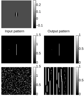
Fig (1) shows the behavior of a subnet for θ = 0, the vertical bars, when the
interactionTijdepends on the orientation ofi−j and isnot rotationally invariant.
Here, Tij > 0between local and roughly vertically displacediand j, and Tij < 0
between local and more horizontally displacedi andj. Hence, two nearby bars i
andjexcite each other when they are co-aligned and inhibit each other otherwise,
as suggested by experimental observations and theoretical studies (e.g., Kapadia et al 1995, Polat and Sagi 1993, Field, Hayes, and Hess 1993). Although the net-work enhances an input (vertical) line relative to the isolated (short) bar, it also hallucinates other vertical lines under noisy inputs.
The competition between internal interactions T and the external inputs I to
shape {xi}is uncompromising in such recurrent networks. For analysis, take for
simplicityTijsuch thatTij 6= 0only wheniandj are in the same or nearest
neigh-bor (vertical) columns. T0 ≡Pj,mj=miTij >0is the total recurrent excitation within
a vertical contour (column) for contour enhancement, andT1 ≡ −Pj,mj=mi+1Tij =
−P
j,mj=mi−1Tij > 0. is the total recurrent suppression between two nearby
ver-tical columns, to suppress noise and background. BothT0 andT1 should be large
for a large difference in saliency between a vertical contour and a homogeneous background input Ii = Ij for all i, j. However, when T0 + 2T1 > 1 (forg0x = 1),
this network under homogeneous input spontaneously breaks symmetry to hallu-cinate saliency waves — two alternate saliencies for neighboring columns. (Math-ematically,T0+ 2T1is the eigenvalue of the matrixTwith this saliency wave as the
eigenvector.) Hence, contour enhancement makes the network prone to “see” con-tours even when there is none. The orientations and widths of the “ghost concon-tours” match the interaction structureT. Avoiding the hallucination forces T0 and/orT1
Local connection Pattern T
Input pattern Output pattern
−0.1 0 0.1 0.2
0 0.5 1 1.5
0 0.5 1 1.5
0 0.5 1
0 0.5 1
Figure 1: A reduced model consisting of symmetrically coupled cells tuned to ver-tical orientation (θ = 0). Shown here are 5 gray scale images, each has a scale bar on
the right. The network has 100x100 cells arranged in a 2-d array, with wrap around boundary condition. Each cell models a cortical cell tuned to vertical orientation, in a retinotopic manner. The sigmoid functiongx(x)of the cells isgx(x) = 0when
x < 1, gx(x) = x−1 when 1 ≤ x < 2, andgx(x) = 1 when x > 2. The top
im-age shows the connection pattern between the center cell and the other cells. This pattern is local and translation invariant, it gives local colinear excitation between cells vertically displaced, and local inhibition between cells horizontally displaced. Middle left: 2-d input patternI, an input line and a noise spot. Middle right: 2-d
output patterngx(x)to the input at middle left — the line induces a response that
is ∼ 100% higher than the noise spot. Bottom left: 2-d input pattern I for noise
input. Bottom right: 2-d output patterngx(x)to the noisy input — hallucination of
vertical streaks.
2.2 A minimal recurrent model with hidden units
The major weakness of the symmetrically connected model is the attractor dynam-ics which strongly attract the network state{xiθ}away from the ones guided by the
visual input{Iiθ}. Since this attractor dynamics is largely dictated by the
spiking neurons (rather than firing rate neurons), for instance, nor by mechanisms like shunting inhibition, global activity normalization, and input gating (Gross-berg and Mingolla 1985, Zucker et al 1989, Braun et al 1994), which are used by many models despite their questionable biological foundations. Attractor dynam-ics is untenable, however, in the face of the well established fact that a real neuron is either exclusively excitatory or exclusively inhibitory. It is obviously impossible to have symmetric connections between excitatory and inhibitory neurons. Math-ematical analysis by Li and Dayan (1999) showed that asymmetric recurrent E-I networks with separate excitatory (E) and inhibitory (I) cells can indeed perform computations that symmetric ones cannot. Thus we model neurons xiθ as
exclu-sively excitatory pyramidal cells, and introduce one inhibitory interneuron (hid-den units) yiθ for each xiθ to mediate indirect, or disynaptic, inhibition between
xiθ’s, as in the real cortex (White 1989, Gilbert 1992, Rocklandand Lund 1983, also
see Grossberg and Raizada 2000 for a much more fully elaborated model). The unitsxiθ andyiθ in such an E-I pair are reciprocally connected. Hence the
dynami-cal equations become: ˙
xiθ = −xiθ−gy(yi,θ) +Jogx(xiθ)−
X
∆θ6=0
ψ(∆θ)gy(yi,θ+∆θ)
+ X
j6=i,θ0
Jiθ,jθ0gx(xjθ0) +Iiθ+Io (5)
˙
yiθ = −αyyiθ +gx(xiθ) +
X
j6=i,θ0
Wiθ,jθ0gx(xjθ0) +Ic (6)
where αy and gy(y)model the interneuron yiθ, which inhibits its partnerxiθ. The
longer range connectionsTiθ,jθ0 (between cells in different hypercolumnsi6=j) are
now separated into two terms: (1) monosynaptic excitationJiθ,jθ0 ≥ 0betweenxiθ
and xjθ0 and (2) disynaptic inhibition Wiθ,jθ0 ≥ 0 between xiθ and xjθ0 via the
in-terneuronyiθ. Including both the monosynaptic and disynaptic pathways, the net
effective connection betweenxiθ and xjθ0 in stationary (but not in dynamic) states
is, for example,Jiθ,jθ0−Wiθ,jθ0/αy ifgy(y) =y, and it can be either facilitatory or
in-hibitory. Bothψ(∆θ)andJo are explicit representations of the original interaction
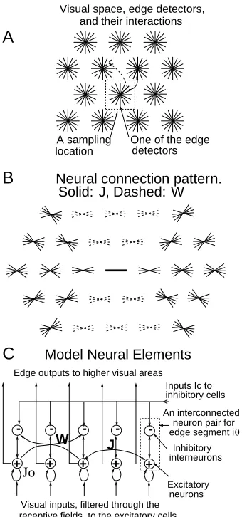
Tiθ,iθ0 between units within a hypercolumn. ψ(∆θ)≤1models local inhibition and Jogx(xiθ)models self excitation. Fig. (2C) schematically shows an example of the
network. IcandIo are background inputs, including neural noise, feedback from
higher areas, and inputs modeling the general and local normalization of activities (Li 1998) (which are omitted in the analysis in this paper, though are present in the simulations). An edge of input strengthIˆiβatiwith orientationβ in the input image contributes toIiθ(forθ≈β) by an amountIˆiβφ(θ−β), whereφ(θ−β)is the
orientation tuning curve.
Lateral connections link cells preferring similar orientations. To implement net colinear facilitation and non-colinear flank inhibition (between similarly ori-ented bars), the excitatoryJconnections are dominant between units preferring
co-aligned bars (θ ∼θ0 ∼6 (i−j)), while the inhibitoryW connections are dominant
A
location
One of the edge A sampling
detectors and their interactions Visual space, edge detectors,
B Neural connection pattern.
Solid: J, Dashed: W
C Model Neural Elements
+
-+
-+
-+
-+
-Jo
W J
Inputs Ic to inhibitory cells
neuron pair for edge segment i
Inhibitory interneurons
Excitatory neurons Edge outputs to higher visual areas
Visual inputs, filtered through the receptive fields, to the excitatory cells.
θ An interconnected
Figure 2: A schematic of the minimal model of the primary visual cortex.A:Visual inputs are sampled in a discrete grid by edge/bar detectors, modeling receptive fields (RFs) for V1 layer 2-3 cells. Each grid point has K neuron pairs (see C),
one per bar segment. All cells at a grid point share the same RF center, but are tuned to different orientations spanning180o, thus modeling a hypercolumn. A bar
segment in one hypercolumn can interact with another in a different hypercolumn via monosynaptic excitation J (the solid arrow from one thick bar to another),
and/or disynaptic inhibitionW (the dashed arrow to a thick dashed bar). See also
C.B: A schematic of the neural connection pattern from the center (thick solid) bar to neighboring bars within a finite distance (a few RF sizes).J’s contacts are shown
by thin solid bars. W’s are shown by thin dashed bars. All bars have the same
connection pattern, suitably translated and rotated from this one. C: An input bar segment is associated with an interconnected pair of excitatory and inhibitory cells, each model cell models abstractly a local group of cells of the same type. The excitatory cell receives visual input and sends outputgx(xiθ)to higher centers.
The inhibitory cell is an interneuron. The visual space has toroidal (wrap-around) boundary conditions.
W > 0for mutual inhibition (Li 1998, 1999a). Physiological evidence (Hirsch and Gilbert 1991) suggests that both Jiθ,jθ0 > 0and Wiθ,jθ0 > 0contribute to the links
between a given pair of pyramidal cells xiθ and xjθ0. This gives extra
computa-tional flexibility (e.g., contrast dependence of contextual influences, see section 3) by letting the ratioJiθ,jθ0 : Wiθ,jθ0 determine the overall sign of the interaction. For
illustrative convenience, however, the simpler bi-phasic connection is sometimes used in this paper to demonstrate our analysis and is used for all the examples in the figures.
As we mentioned, in principle, an E-I recurrent model can perform computa-tions that symmetric models cannot. In practice, this is not guaranteed and has to be ensured by designing the right model parameters, in particular, J and W,
guided by an analytical understanding of the nonlinear dynamics.
3 Dynamic analysis
x
g (x)
cell membrane potential
Cell firing rate x
Activation function for excitatory cells
cell membrane potential
Cell firing rate y
Activation function for inhibitory cells
g (y)y
g (x) x input at different Ic
For lower Ic
Edge response to visual
Input I to the excitatory cell
Edge response
For higher Ic
Ι c Ι Ι c
Ι
= g’ (y)
y
I
This region for input suppression for input
This region
facilitation
curve on which
A
B
C
D
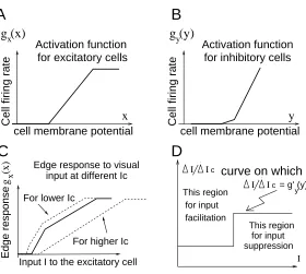
Figure 3: A,B: examples of gx(x) and gy(y) functions. C: Input-output function
I →gx(¯x)for an isolated neural pair without inter-pair neural interactions, under
different levels of Ic. D: The overall effect of the external or contextual inputs
(∆I,∆Ic) on a neural pair is excitatory or inhibitory if∆I/∆Icis large or less than
g0
y(¯y), which depends onI.
The model state is characterized by{xiθ, yiθ}, or simply{xiθ}, omitting the
hid-den units {yiθ}. The interaction between excitatory and inhibitory cells makes
{xiθ(t)}intrinsically oscillatory in time. Given an input {Iiθ}, the model does not
converges to, or oscillates periodically around, a fixed point, after the transient fol-lowing the onset of {Iiθ}, the temporal average {¯xiθ} of {xiθ(t)} can characterize
the model output and approximate the fixed point. We henceforth use the nota-tion{¯xiθ}to denote either the fixed point or the temporal average, and denote the
computation as I → gx(¯xiθ). Section 3.1-3.6 will analyze I → gx(¯xiθ) and derive
constraints onJ andW in order to makeI →gx(¯xiθ)achieve the desired
computa-tions. Other investigators have also analyzed the fixed point behaviorI →gx(¯xiθ)
in such E-I networks or the corresponding symmetric ones (Ben-Yishai et al 1995, Stemmler et al 1995, Somers et al 1998, Mundel et al 1997, Tsodyks et al 1997), mainly to model a local circuit of a hypercolumn (or a CA1 region) with simplified or no spatial organization beyond the hypercolumn. Our analysis emphasizes the spatial or geometrical organization of visual inputs in order to study global visual computations. Section 3.7 studies the stability and dynamics around{x¯iθ}and
de-rives constraints on the model parameters coming from the need to avoid visual hallucination (Ermontrout and Cowan 1979) — the curse of symmetric networks.
3.1 A single pair of neurons
In isolation, a single pairiθfollows equations
˙
x = −x−gy(y) +Jogx(x) +I (7)
˙
y = −y+gx(x) +Ic (8)
where αy = 1 for simplicity (as in the rest of the paper), index iθ is omitted, and
I =Iiθ +Io. The input-output (I, Ic→gx(¯x)) gain at a fixed point(¯x,y¯)is
δgx(¯x)
δI =
g0
x(¯x)
1 +g0
x(¯x)gy0(¯y)−Jog0x(¯x)
, δgx(¯x) δIc
=−g0
y(¯y)
δgx(¯x)
δI (9)
When both gx(x)and gy(y)are piece-wise linear (Fig. (3A,B)) functions, so is the
input-output relationI → gx(¯x)(Fig. (3C)). The threshold, input gain control, and
saturation in I → gx(¯x)are apparent. The slope δgδIx(¯x) is non-negative, otherwise,
I = 0 gives non-zero output x 6= 0. It increases withg0
x(¯x), decreases with gy0(¯y),
and depends onIc. Shifting(I, Ic)to(I+ ∆I, Ic+ ∆Ic)changesgx(¯x)by∆gx(¯x)≈
(δgx(¯x)/δI)(∆I −gy0(¯y)∆Ic), which is positive or negative depending on whether
∆I/∆Ic > gy0(¯y). Hence, a more elaborate model could allow a fraction of the
external visual input to go onto interneurons, as suggested by physiology (White 1989) and modeled by Grossberg and Raizada (2000), provided that ∆I/∆Ic >
g0
y(¯y). Contextual inputs from other neuron pairs (via J and W) effectively give
(∆I,∆Ic). In our example whengy0(¯y)increases withI (orIc), the contextual inputs
can switch from being facilitatory to being suppressive asI increases (Fig. (3 D)).
3.2 Two interacting pairs of neurons with non-overlapping
recep-tive fields
Using indicesa= 1,2to denote the two pairs and their associated quantities (J12=
J21=J andW12=W21 =W),
˙
xa = −xa−gy(ya) +Jogx(xa) +Jgx(xb) +Ia+Io
˙
ya = −ya+gx(xa) +W gx(xb) +Ic
wherea, b= 1,2anda6=b. Including monosynaptic and disynaptic pathways, the
net effective connection from x2 to x1, according to the gain functions δgx(¯x)/δI
andδgx(¯x)/δIc, isJ−gy0(¯y1)W. WhenI ≡I1 =I2in the simplest case,x¯≡x¯1 = ¯x2
and y¯ ≡ y¯1 = ¯y2. The two bars can excite or inhibit each other depending on
whether J − g0
y(¯y)W > 0. This in turn depends on the input I through gy0(¯y).
When I1 > I2, we have (¯x1,y¯1) > (¯x2,y¯2). Usually, gy0(¯y) increases with y¯, hence
J12−gy0(¯y1)W12< J21−gy0(¯y2)W21. In particular, it can happen thatJ12−gy0(¯y1)W12<
0 < J21−gy0(¯y2)W21, i.e., x1 excitesx2 which in turn inhibits x1. This implies that
two interacting pairs tend to have closer activity valuesx1 and x2 than two
non-interacting pairs.
Even this very simple contextual influence can already account for some per-ceptual phenomena involving sparse visual inputs consisting only of single test and contextual bars. Examples include the altered detection threshold (Polat and Sagi 1993, Kapadia et al 1995) or perceived orientation (tilt illusion, Mundel et al 1997, Kapadia 1998) of a test bar when a contextual bar is present.
3.3 A one dimensional array of identical bars
An infinitely long, horizontal array of evenly spaced, identical, bars gives an input pattern approximated as
Iiθ =
(
Iarray fori= (mi, ni = 0)on the horizontal axis andθ =θ1
0 otherwise (10)
The approximation Iiθ = 0 forθ 6= θ1 is good for small orientation tuning width
and low input contrast. When bars iθ outside that array are silent gx(xiθ) = 0
due to insufficient excitation, we omit them and treat the remaining system as one dimensional. Omitting index θ and usingi to denote bars according to their one
dimensional location, we get ˙
xi = −xi−gy(yi) +Jogx(xi) +
X
j6=i
Jijgx(xj) +Iarray+Io (11)
˙
yi = −yi+gx(xi) +
X
j6=i
Wijgx(xj) +Ic (12)
Translation symmetry implies that all units have the same equilibrium point (¯xi,y¯i) = (¯x,y¯), and
˙¯
x = 0 =−¯x−gy(¯y) + (Jo+
X
i6=j
D
E
θ1
A
C
B
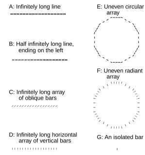
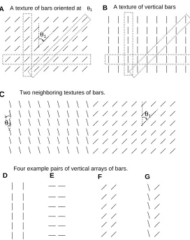
Figure 4: Examples of the one dimensional input stimuli mentioned in the text. A: horizontal array of identical bars oriented at angle θ1. B: A special case of A
when θ1 = π/2and, in C, when θ1 = 0. D: an array of bars aligned into, or
tan-gential to, a circle, the pattern in Bis a special case of this circle when the radius is infinitely large. E: same as D except that the bars are perpendicular to the circle circumference, the pattern inCis a special case when the radius is infinitely large.
˙¯
y = 0 =−¯y+ (1 +X
i6=j
Wij)gx(¯x) +Ic (14)
This array is then equivalent to a single neural pair (cf. equations (7) and (8)) with the substitutionJo → Jo+PjJij and g0(¯y) → gy0(¯y)(1 +
P
jWij). The response to
bars in the array is thus higher than that to an isolated bar if the net extra excitatory connection
E ≡X
j
Jij (15)
is stronger than the net extra inhibitory (effective) connection I ≡g0
y(¯y)
X
j
Wij. (16)
The input-output relationshipI →gx(¯x)is qualitatively the same as that of a single
bar, with a quantitative change in the gain
δgx(¯x)
δI =
g0
x(¯x)
1 +g0
x(¯x)(gy0(¯y)−(E − I))−Jogx0(¯x)
. (17)
EandIdepend onθ1. Consider the case of association field connections. When the
bars are parallel to the array, making a straight line (Fig (4B)),E >I. The condition
for contour enhancement is
A: Infinitely long line
B: Half infinitely long line, ending on the left
C: Infinitely long array of oblique bars
D: Infinitely long horizontal array of vertical bars
E: Uneven circular array
F: Uneven radiant array
G: An isolated bar
Figure 5: Simulated outputs from a cortical model to corresponding visual input patterns of 1 dimensional arrays of bars. The model transforms input Iiθ to cell
outputgx(xiθ). The thicknesses of the barsiθ are proportional to temporally
aver-aged model outputsgx(xiθ). The corresponding (suprathreshold) inputIˆiθ = 1.5is
of low/intermediate contrast and is the same for all 7 examples and all visible bars. Different outputsgx(xiθ)for different examples or for different bars in each
exam-ple are caused by contextual interactions. Overall contextual facilitations cause higher outputs inA, B, Ethan that of an isolated bar inG, while overall contextual suppressions cause lower outputs inC, D, F(compare the different thicknesses of the bars). Note the deviations from the idealized approximations in the text. Un-even spacing between the bars (F, G) or an end of a line (at the left end ofB) cause deviations from the translation invariance of responses. Note that the responses taper off near the line end in B, and that the responses are noticably weaker to bars that are more densely packed in F. InA, B, cells preferring neighboring ori-entations (near horizontal) at the line are also excited above threshold, unlike the approximated treatment in the text.
When the bars are orthogonal to the array ( Fig (4C)),E <Iand the responses are suppressed. This analysis extends to other translation invariant one dimensional arrays like those in Fig (4D, E), for which the index i simply denotes a bar at a
location along the array (Li 1998). The straight line in Fig (4B) is in fact the limit of a circle in Fig (4D) when the radius goes to infinity. Similarly, the pattern in Fig (4C) is a special case of the one in Fig (4E).
in-put, as shown in Fig. (5). Contextual facilitation in Fig. (5A, B, E) and contextual suppression in Fig. (5C, D, F) are visualized by the thicker and thinner bars, re-spectively, than the isolated bar in Fig. (5G). In Fig. (5A), cells whose RFs are centered on the line but not oriented exactly horizontally are also excited above threshold, unlike our approximationgx(xiθ) = 0for non-horizontalθ. (This should
not cause perceptual problems, though, given population coding.) This is caused by direct visual inputIiθ forθ 6=θ1 (θ ≈ θ1)andthe colinear facilitation from other
bars in the line. The approximation of translation invariancex¯i = ¯xj for all bars in
the array is compromised when the array has an end, e.g., Fig. (5B), or when the bars are unevenly spaced, e.g., Fig. (5E,F). In Fig. (5B), the bars at or near the left end of the line are less enhanced since they receive less or no contextual facilitation from their left. In Fig. (5F), the more densely spaced bars receive more contextual suppression than others.
3.4 Two dimensional textures and texture boundaries
The analysis of the one dimensional array also applies to an infinitely large two dimensional texture of uniform inputIiθ1 =Itexturewheni= (mi, ni)sit on a
regu-larly spaced grid (Fig. (6A)). The sumsE = P
jJij andI = g0y(¯y)
P
jWij are taken
over allj in that grid.
Physiologically the response to a bar is reduced when the bar is part of a texture (Knierim and van Essen 1992). This can be achieved when E < I. Consider, for
example, the case when i = (mi, ni) form a Manhattan grid with integer values
of mi and ni (Fig (6)). The texture can be seen as a horizontal array of vertical
arrays of bars, e.g., a horizontal array of vertical contours in Fig. (6B). The effective connections between the vertical arrays (Fig. (6DEF)) distanceaapart are:
Ja0 ≡ X
j,mj=mi+a
Jij, Wa0 ≡
X
j,mj=mi+a
Wij. (19)
Then E = P
aJa0 and I = gy0(¯y)
P
aWa0. The effective connection within a single
vertical array isJ0
0andW00. One has to designJandW such that contour
enhance-ment and texture suppression can occur using the same neural circuit (V1). That is, when the vertical array is a long straight line (θ1 = 0), contour enhancement
(i.e., J0
0 > gy0(¯y)W00) occurs when the line is isolated, but overall suppression (i.e.,
E = P
aJa0 < I = gy0(¯y)
P
aWa0) occurs when that line is embedded within a
tex-ture of lines (Fig. (6B)), as long as there is sufficient excitation within a line and sufficient inhibition between the lines.
Computationally, contextual suppression within a texture means that the boundaries of a texture region induce relatively higher responses, thereby mark-ing the boundaries for segmentation. The contextual suppression of a bar within a texture is
Cθ1
whole−texture ≡
X
a
(g0
y(¯yθ1)W
0θ1
a −Ja0θ1)gx(¯xθ1) = (I − E)gx(¯xθ1)>0 (20)
wherex¯θ1 denotes the (translation invariant) fixed point for all texture bars.
B
F G
E D
A texture of vertical bars
Two neighboring textures of bars.
Four example pairs of vertical arrays of bars.
A A texture of bars oriented at
θ2
θ1 θ1
θ1
C
Figure 6: Examples of the two dimensional textures and their interactions. A: tex-ture made of bars oriented atθ1 and sitting on a Manhattan grid. This can be seen
as a horizontal array of vertical array of bars. B: a special case ofAwhen θ1 = 0.
This is a horizontal array of vertical lines. Each texture can also be seen as a ver-tical array of horizontal arrays of bars, or an oblique array of oblique arrays of bars. Each vertical, horizontal, or oblique array can be viewed as a single entity, shown as examples in the dotted boxes. C: Two nearby textures and the bound-ary between them. D, E, F: examples of nearby and identical vertical arrays. G: two nearby but different vertical arrays. When each vertical array is seen as an en-tity, one can calculate effective connectionsJ0andW0(defined in the text) between
these vertical arrays.
lefti = (mi < 0, ni) removes the contextual suppression from them, and so gives
them higher responses. This highlights the texture boundary mi = 0. Now the
activityx¯iθ1 depends onmi, i.e., the distance of the bars from the texture boundary.
Asmi → ∞, x¯iθ1 → x¯θ1. The contextual suppression of the bars on the boundary,
mi = 0, is
Cθ1
half−texture ≡
X
mj≥0
(g0
y(¯yiθ1)W
0θ1
mj −J 0θ1
mj)gx(¯xjθ1) (21)
≈ X
a≥0
(gy0(¯yθ1)W
0θ1
a −J
0θ1
a )gx(¯xθ1)< C
θ1
A B
C D
Input
Output
Input
Output
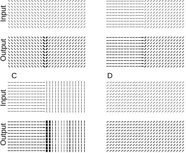
Figure 7: Simulated examples of texture boundary highlights between different pairs of textures, defined by bar orientations. In each example, we show the input image Iiθ above the output image gx(xiθ) averaged in time. Each image shows
a small region out of an extended input area. A: θ1 = 45o, θ2 = −45o. B: θ1 =
45o, θ
2 = 90o. C: θ1 = 0o, θ2 = 90o. D: θ1 = 45o, θ2 = 60o. The texture border
is vertical in the middle of each stimulus pattern. Note how border highlights increase with increasing orientation contrastθ1−θ2. The orientation contrast of15o
inDis difficult to detect by the model or humans. The orientation contrastθ1−θ2 =
90ofor bothAandC. Note how the responses to the boundary bars decrease with
increasing orientation differences between the bars and the boundary.
where we approximate(¯xjθ1,y¯jθ1)≈(¯xθ1,y¯θ1)for allmj ≥0.
The boundary highlight persists when a neighboring, different, texture of bars oriented at θ2 for i = (mi < 0, ni) is present (Fig. (6C)). To analyze this, define
connections between arrays in different textures (Fig. (6G)) as
J0θ1θ2
a ≡
X
j,mj=mi+a
Jiθ1jθ2 W
0θ1θ2
a ≡
X
j,mj=mi+a
Wiθ1jθ2 (23)
Whenθ1 =θ2,Ja0θ1θ2 =Ja0θ1 andWa0θ1θ2 =Wa0θ1. The contextual suppression from the
neighboring texture (θ2) on the texture boundary (mi = 0) isCneighborθ1,θ2 −half−texture ≡
P
mj<0(g 0
y(¯yiθ1)W
0θ1θ2
mj − J 0θ1θ2
mj )gx(¯xjθ2). For the association field connection, Jiθ1,jθ2
andWiθ1,jθ2 tend to link similarly oriented barsθ1 ∼θ2, we haveC
θ1,θ2
neighbor−half−texture
minimum or zero when θ1 ⊥ θ2 and increasing with decreasing|θ1 −θ2|. Hence,
the boundary highlight is expected to increase with the orientation contrast |θ1 −
θ2|. The net contextual suppression on the border, contributed by both textures, is
Cθ1,θ2
2−half−textures ≡Chalfθ1 −texture+C
θ1,θ2
neighbor−half−texture. Hence, the border enhancement,
or the reduction of contextual suppression at the border relative to regions further inside the texture is
δC ≡ Cθ1
whole−texture−C
θ1,θ2
≈ Cθ1,θ2=θ1
neighbor−half−texture−C
θ1,θ2
neighbor−half−texture (25)
≈ X
a<0
(g0y(¯yθ1)W
0θ1
a −Ja0θ1)gx(¯xθ1)−
X
a<0
(gy0(¯yθ1)W
0θ1θ2
a −Ja0θ1θ2)gx(¯xθ2) (26)
Again, we made the approximationx¯jθ2 ≈x¯θ2 formj <0. Usuallyx¯θ2 6= ¯xθ1 since
the fixed point should depend on the relative orientation between the bars and the arrays (i.e., the axes). AssumingJ0θ1θ2
a ≈ 0 and Wa0θ1θ2 ≈ 0when |θ1 −θ2| = π/2,
and noting thatx¯θ1 ≈x¯θ2 whenθ1 ≈θ2,
δC ≈
0 forθ1 ≈θ2
P
a<0(gy0(¯yθ1)W
0θ1
a −Ja0θ1)gx(¯xθ1)>0 forθ1 ⊥θ2
roughly increases as|θ1−θ2|increases
(27)
Thus the border highlight diminishes as the orientation contrast approaches0, see Fig. (7). Furthermore, even at a given contrast |θ1 −θ2|, the border enhancement
δC depends on θ1. For instance, with |θ1 − θ2| = π/2 and the association field
connections, the enhancement δC for border bars parallel to the border θ1 = 0
(which form a contour) is higher than that for border bars perpendicular to the borderθ1 = π/2. This is because both the suppressiongy0(¯yθ1)W
0θ1
a −Ja0θ1 between
parallel contours (θ1 = 0 and a 6= 0) and the facilitation J00θ1 −gy0(¯yθ1)W
0θ1
0 within
a contour (Fig. (6D)) are much stronger than their counterparts for the vertical arrays of horizontal bars (Fig. (6E)). Thus the strength of the border highlight is predicted to be tuned to the relative orientationθ1between the border and the bars
(Li 2000). This explains the asymmetry in the outputs of Fig. (7C), the highlight of the vertical border is much stronger for the vertical than the horizontal texture bars.
Clearly, the approximations x¯iθ1 ≈ x¯θ1 formi ≥ 0 and x¯iθ2 ≈ x¯θ2 for mi < 0),
which are used to arrive at equation (27), break down at the border, especially at more salient borders like that in Fig. 7C. This accentuates the tuning of the border highlight toθ1.
Iso-orientation suppression underlies the border highlight, and by equation (20), its strengthI − E depends on contrast through g0
y(¯y). Sincegy0(¯y)usually
in-creases with increasingy¯, the highlight is stronger at higher contrast. Psychophys-ically, texture segmentation does require an input contrast well above the texture detection threshold (Nothdurft 1994). It is easy to tune the connection weights in the model quantitatively such that iso-orientation suppression holds at all input contrasts, or holds only at sufficient input contrast and becomes iso-orientation fa-cilitation at very low contrast as in Li (1998, 1999a). Computationally, fafa-cilitation certainly helps texture detection, which at low input contrast could be more im-portant than segmentation. On this note, contour facilitation (Fcontour >0) holds at
all contrasts (Li 1998) using the bi-phasic connection, since no W connections link the contour segments. Non-bi-phasic connections should be employed to model diminished contour enhancement at high contrast (Sceniak et al 1999).
3.5 Translation invariance and pop-out
A B C
Figure 8: Model responses to homogeneous (A, B) and inhomogeneous (C) input images, each composed of bars of equal input contrasts. A:A homogeneous (de-spite of the orientation contrast) texture of bars of different orientations, a uniform output saliency results. B: Another homogeneous texture, vertical bars are more salient, however the whole texture has a translation invariant saliency distribution. C:The small figure pops out from the background because it is where translation invariance is broken in inputs, and the whole figure is its own boundary.
if orientation contrasts are homogeneous within the texture itself, they will not pop out. Fig. (8A) shows an example for which the texture is made of alternat-ing columns of bars at θ1 = 45o (even a) and θ2 = 135o (odd a). The contextual
suppression of a bar oriented atθ1 is:
Ccomplex−texture =
X
evena(g 0
y(¯yθ1)W
0θ1
a −Ja0θ1)gx(¯xθ1)+
X
odda
(g0
y(¯yθ1)W
0θ1θ2
a −Ja0θ1θ2)gx(¯xθ2)
(28) Thus no bar oriented atθ1 is less suppressed, or more salient, than other bars
ori-ented at θ1. Note that since Ccomplex−texture 6= Cwholeθ1 −texture, the value of x¯θ1 is not
the same as it would be in a simple texture of bars of a single orientationθ1. This
applies similarly tox¯θ2. For generalθ1 and θ2, x¯θ1 6= ¯xθ2. In Fig. (8A), reflection
symmetry leads to x¯θ1 = ¯xθ2 or uniform saliency within the whole texture. In
Fig. (8B), bars oriented atθ1 = 0o induced higher responses than those oriented at
θ2 = 90o. Nevertheless, looking at this texture which is defined by both the vertical
and horizontal bars and their spatial arrangement, no local patch of the texture is more salient than any other patch. This translation invariance in saliency is simply the result of the network preserving the translation invariance in the input (tex-ture), as long as the translation symmetry is not spontaneously broken (see section 3.7 for analysis).
3.6 Filling-in and leaking-out
Small fragments of a contour or homogeneous texture can be missing in inputs due to input noise or to the visual scene itself. Filling-in is the phenomenon that the missing input fragments are not noticed, see Pessoa Thompson, and Noe (1998) for an extensive discussion. It could be caused by one of the following two possi-ble mechanisms. The first is that, although the cells for the missing fragment do not receive direct visual inputs, they are excited enough by the contextual influ-ences to fire as if there were direct visual inputs. (This is how (e.g.,) Grossberg and Mingolla (1985) model illusory contours.) The second possibility is that, even though the cells for the missing fragment do not fire, the regions near, but not at, the missing fragments are not salient or conspicuous enough to attract visual attention strongly. In the latter case, the missing fragments are only noticable by at-tentive visual scrutiny/search. It is not clear from physiology (Kapadia et al 1995) which mechanism is involved.
A B
Input
Output
Figure 9: Examples of filling-in — model outputs from inputs composed of bars of equal contrasts in each example. A:A line with a gap, the response to the gap is non-zero,B:A texture with missing bars, the responses to bars near the missing bars are not significantly higher than the responses to other texture bars.
Consider a single bar segmenti= (mi = 0, ni = 0)missing in a smooth contour,
say, a horizontal line like Fig. (9A), filling-in could be achieved by either of the two possible mechanisms. To excite the cell ito firing threshold Tx (such thatgx(xi >
Tx)>0), contextual facilitationPj(Jij−Wijgy0(¯yi))gx(¯xj)should be strong enough,
or approximately
whereIo is the background input, Fcontour and the effective net connectionsE and
I are as defined in equations (15 - 18), and we approximate for all contour bars (¯xj,y¯j) by (¯x,y¯), the translation invariant activity in a complete contour. If
seg-ments within a smooth contour facilitate each other’s firing, then a missing frag-ment i reduces the saliencies of the neighboring contour segments j ≈ i. The
missing segment and its vicinity are thus not easily noticed, even if the cell i for
the missing segment does not fire.
The celli= (mi = 0;ni = 0)should not be excited enough to fire if the left half
j = (mj <0, nj = 0)of the horizontal contour are removed. Otherwise the contour
extends beyond its end or grows in length — leaking out. To prevent leaking-out
Fcontour/2 +Io < Tx (30)
since the contour facilitation to i is approximately Fcontour/2, half of that Fcontour
in an infinitely long contour. The inequality (30) is satisfied for the line end in Fig. (5B), and should hold at any contour saliency gx(¯x). Not leaking out also
means that large gaps in lines can not be filled in. To prevent leaking-out at i = (mi = 0, ni = 1), the side of an infinitely long (e.g.,) horizontal contour on the
horizontal axis in Fig. (4B) (thus to prevent the contour getting thicker), we require
P
j∈contour(Jij−gy0(¯yi)Wij)gx(¯x)< Tx−Iofori6∈contour. This condition is satisfied
in Fig. (5A).
Filling-in in a texture with missing fragments i(texture filling-in) is only
fea-sible by the second mechanism — to avoid conspicuousness near i— since ican
not be excited to fire if contextual input within a texture is suppressive. If i is
not missing, its neighbor k ≈ i receives contextual suppression (I − E)gx(¯x) ≡
P
j∈texture(gy0(¯y)Wkj −Jkj)gx(¯x). A missing imakes its neighbork more salient by
the removal of its contribution(Wkigy0(¯y)−Jki)gx(¯x)to the suppression. This
con-tribution should be a negligible fraction of the total suppression to ensure that the neighbors are not too conspicuous, i.e.,
g0
y(¯y)Wki−Jki (I − E)≡
X
j∈texture
(g0
y(¯y)Wkj −Jkj). (31)
This is expected when the lateral connections are extensive enough to reach suffi-ciently large contextual areas, i.e., whenWki PjWkj andJki PjJkj.
Leaking-out is not expected Leaking-outside a texture border when the contextual input from the texture is suppressive.
Note that filling-in by exciting the cells for a gap in a contour (equation (29)) works against preventing leaking-out (equation (30)) from contour ends. It is not difficult to build a model that achieves active filling-in. However, preventing the model from leaking-out and unwarranted illusory contours implies a small range of choices for the connection strengthsJ andW.
3.7 Hallucination prevention, and neural oscillations
to the actual model behavior. (We use bold-faced character to represent vectors or matrices.) Section 2 showed that this is difficult to achieve in the symmetric net-works, as the fixed points(X¯)for the desired computation are likely to be unstable,
i.e., they are saddle points or local maximums in the energy function. In that case, the actual model output deviates drastically from the desired fixed point(X¯)or
vi-sual input, and, in particular, vivi-sual hallucinations occur. In the corresponding E-I network, the asymmetric connections between E and I give the network a tendency to oscillation around the fixed point. This oscillation enables our model to avoid the motion of(X,Y)towards hallucination (Li and Dayan 1999), making it
possi-ble to correspond the desired fixed points (X¯,Y¯) with the (temporally averaged)
model behavior. However, this correspondence is not guaranteed, and is in fact difficult to achieve without guided model design. It requires stability conditions on(X¯,Y¯)to be satisfied, which constrainsJ and W, in addition to the conditions
placed on J and W in section 3.1-3.6 for desired contour integration and texture
segmentation (the inequalities (18), (20), (29), (30), and (31)). This section derives these stability constraints and their implications. Specifically, we derive the con-dition to prevent visual hallucinations or spontaneous formations of spatially in-homogeneous outputs given translation invariant visual inputs. Ermontrout and Cowan (1979) have analyzed the stability conditions to obtain hallucinations in a simplified model of V1 (see Bressloff et al (2000) for a more recent analysis), and studied the forms and dynamics of the hallucinations. Li (1998) analyzed the sta-bility constraints to prevent hallucination under contour inputs. Here we general-ize the analysis in Li (1998) to other homogeneous inputs, and in addition analyze the nonlinear dynamics of (non-hallucinating) homogeneous oscillations around (X¯,Y¯). We omit the analysis of the emergent hallucinations since the
hallucina-tions are prevented by the model.
To analyze stability, we study how small deviations (X−X¯,Y−Y¯)from the
fixed point evolve. Change variables(X−X¯,Y−Y¯)→(X,Y). For small
devia-tionX,Y, a Taylor expansion on equations (5) and (6) gives the linear
approxima-tion:
˙ X
˙ Y
!
= −1 +J −G
0
y
G0
x+W −1
!
X Y
!
(32) whereJ, W, G0
x, and G
0
y are matrices withJiθjθ0 = Jiθjθ0gx0(¯xjθ0)fori 6= j, Jiθ,iθ = Jogx0(¯xiθ), Wiθjθ0 = Wiθjθ0gx0(¯xjθ0)fori 6= j, Wiθ,iθ0 = 0, G0xiθjθ0 = δiθjθ0gx0(¯xjθ0). and
G0
yiθjθ0 = δijψ(θ−θ 0)g0
y(¯yjθ0)whereψ(0) = 1. To focus on the outputX, eliminate
(hidden) variableY: ¨
X+ (2−J)X˙ + (G0
y(G
0
x+W) +1−J)X = 0 (33)
Consider inputs of our interest which are bars arranged in a translation invari-ant fashion along a one or two dimensional array. For simplicity and approxi-mation, we again omit bars outside the array and their associated quantities in equation (33), and omit the indexθ, like we did in section 3.3 and 3.4. Translation
symmetry implies (¯xi,y¯i) = (¯x,y¯), G0yij = δijg
0
y(¯y), G0xij = δijgx0(¯x), (G0yG
0
x)ij =
g0
x(¯x)gy0(¯y)δij, and (G0yW)ij = gy0(¯y)Wij. Furthermore, Jij = Ji+a,j+a ≡ Ji−j and
spatial variables{Xi}and their associated quantitiesJ,Wto obtain:
¨
Xk+ (2−J) ˙Xk+ (gy0(¯y)(g0x(¯x) +Wk) + 1− Jk)Xk= 0 (34)
where Xk,Jk,Wk are spatial Fourier transforms ofX,J,W for frequency fk such
thateifkN = 1, whereN is the size of the system. X
k is the amplitude of the spatial
wave of frequencyfkin the deviationXfrom the fixed point,Jk=PaJaeifka, and
Wk=PaWaeifka. Xk evolves asXk(t)∝eγkt where
γk ≡ −1 +Jk/2±i
q
g0
y(g0x+Wk)− Jk2/4 (35)
Denote Re(γk) as the real part of γk, Re(γk) < 0 for allk makes any deviationX
decay to zero, and hence no hallucination can occur. Otherwise, the mode with the largestRe(γk), let it be k = 1, will dominate the deviation X(t). If this mode has
zero spatial frequencyf1 = 0, then the dominant deviation is translation invariant
and synchronized across space, and hence no spatially varying patterns can be hallucinated. Thus the conditions to prevent hallucinations are
Re(γk)<0 for allk, or Re(γ1)f1=0 > Re(γk)fk6=0 (36)
WhenRe(γ1)f1=0 >0, the fixed point is not stable, the divergent homogeneous
deviation X is eventually confined by the threshold and saturation nonlinearity.
It oscillates (synchronously) in time wheng0
y(gx0 +W1)− J12/4 > 0or when there
is no other fixed point to which the system trajectory can approach. Denote this translation invariant oscillatory trajectory by(x, y) = (xi, yi), which is the same for
alli. Then,
˙
x = −x−(gy(y+ ¯y)−gy(¯y)) +J1(gx(x+ ¯x)−gx(¯x))
˙
y = −y+ (1 +W1)(gx(x+ ¯x)−gx(¯x))
where J1 = J1/g0
x(¯x)and W1 = W1/gx0(¯x). After converging to a finite oscillation
amplitude, the trajectory(x(t), y(t))is a closed curve in the(x, y)space. It oscillates with periodT such that(x(t+T), y(t+T)) = (x(t), y(t)), and satisfies
Z T
0 dt[(1+
W1)x(gx(x+¯x)−gx(¯x))+y(gy(y+¯y)−gy(¯y))] =
Z T
0 dt
J1(1+W1)(gx(x+¯x)−gx(¯x))2,
(37) since over a cycle of the oscillation, the oscillation energy
Z x+¯x
¯
x (1 +
W1)(gx(s)−gx(¯x))ds+
Z y+¯y
¯
y (gy(s)−gy(¯y))ds, (38)
dissipation dominates because of the saturation and/or threshold behavior in self-excitation. Thus the oscillation trajectory converges to the balance of a periodic nonlinear oscillation.
SinceJa =J−a ≥0andWa =W−a ≥ 0,Jk andWkare real and have maxima
M ax(Jk) = PaJa and M ax(Wk) = PaWa for the zero frequency fk = 0 mode.
Many simple forms of J and W decay with fk, for example, Ja ∝ e−a2/2
gives Jk ∝ e−f
2
k/2. However, the dominant mode is determined by the value ofRe(γk),
and may have f1 6= 0. In principle, given a model interaction J and W and a
translation invariant input, whether it is arranged on a Manhattan grid or some other grid, Re(γk) should be evaluated for all k to ensure appropriate behavior
of the model or inequalities (36). In practice, the finite range of (J, W) and the
discreteness and the (rotational) symmetry in the image grid implies that often only a finite, discrete, set ofkneeds to be examined.
Let us look at some examples using the bi-phasic connections. For 1-d contour input like that in Fig. (4B),Wij = 0. ThenRe(γk) =Re(−1 +Jk/2±i
q
g0
ygx0 − Jk2/4)
increases with Jk, whose maximum occurs at the translation invariant mode
f1 = 0, andJ1 = PjJij. Then no hallucination can happen, though synchronous
oscillations can occur when enough excitatory connections J link the units
in-volved. For 1-d non-contour inputs like Fig. (4C,E),Jij = 0fori6=j, thusJk =Jii,
γk =−1+Jii/2±i
q
g0
y(g0x+Wk)−J2ii/4. HenceRe(γk)<−1+Jii=−1+Jogx0(¯x)<0
for allk, since−1 +Jogx0(¯x)<0is always satisfied (otherwise an isolated principal
unitx, which follows equationx˙ =−x+Jxgx(x) +I, is not well behaved). Hence
there should be no hallucination or oscillation.
Under 2-dimensional texture inputs, frequency fk = (fx(k), fy(k)) is a wave
vector perpendicular to the peaks and troughs of the waves. Whenfk = (fx(k),0)
is in the horizontal direction,Jk = g0(¯x)PaJa0eifx(k)a andWk = g0(¯x)PaWa0eifx(k)a,
whereJ0
aandWa0 are the effective connections between two texture columns as
de-fined in equation (19). Hence, the texture can be analyzed as a 1-dimensional array as above, substituting bar-to-bar connections(J, W)by column-to-column connec-tions (J0, W0). However, J0 and W0 are stronger, have a more complex Fourier
spectrum (Jk,Wk), and depend on the orientation θ1 of the texture bars. Again
use the bi-phasic connection for examples. When θ1 = 90o (horizontal bars), Wb0
is weak between columns, i.e.,W0
b ≈ δb0W00 andWk ≈ W00. Then,Re(γk)is largest
whenJkis, at fx(k) = 0— a translation invariant mode. Hence, illusory saliency
waves (peaks and troughs) perpendicular to the texture bars are unlikely. Con-sider however vertical texture bars for the horizontal wave vectorfk = (fx(k),0).
The bi-phasic connection gives nontrivialJ0
b and Wb0 between vertical columns, or
non-trivial dependences ofJk andWkonfk. The dominant mode with the largest
Re(γk)is not guaranteed to be homogeneous, andJ andW must be tuned in order
to prevent hallucination.
Given a non-hallucinating system and under simple or translation invariant inputs, neural oscillations, if they occur, can only be synchronous and homo-geneous (i.e., identical) among the units involved, i.e., f1 = 0. Since γ1 =
−1 +J1/2±i
q
g0
y(gx0 +W1)− J12/4, andJ1 =PjJijforf1 = 0, the tendency for
Model input pattern Cell temporal activities
A
B
C
D
0 0.2 0.4 0.6 0.8 1
Outputs for isolated bar
0 0.2 0.4 0.6 0.8 1
Outputs for 2 line segments
0 0.2 0.4 0.6 0.8 1
Outputs for 2 array bars
0 1 2 3 4 5 6 7 8 9 10
0 0.2 0.4 0.6 0.8 1
time
Outputs for 3 texture bars
involved (Koenig and Schillen 1991). Hence, this tendency is likely to be higher for 2-d texture inputs than for 1-d array inputs, and lowest for a single, small, bar in-put. This may explain why neural oscillations are observed in some physiological experiments and not others. Under the bi-phasic connections, a long contour input is more likely to induce oscillation than an input of non-contour 1-d array, see Fig. (10). These predictions can be physiologically tested. Indeed, physiologically, grat-ing stimuli are more likely to induce oscillations than bar stimuli (Molotchnikoff, Shumikhina, and Moisan, 1996).
4 Summary and Discussion
In this paper, we have argued that a recurrent model composed of interacting E-I pairs is a suitable minimal model of the primary visual cortex performing pre-attentive computation of contour integration and texture segmentation. We ana-lyze the nonlinear input-output transform I → gx(x) and the stability and
tem-poral dynamics of the model. We derived design conditions on the intracortical connections such that (1) I → gx(x) performs the desired computations, and (2)
no hallucinations occur. Such an understanding has been essential to reveal the computational potential and limitations of the models, and led to a successful de-sign (Li 1998, 1999a). The analysis techniques in this paper can be applied to other recurrent networks whose neural connections are translationally symmetric.
Note that the design conditions for a functional model can be satisfied by many quantitatively different models with qualitatively the same architecture. The model by Li (1998, 1999a) is one of them, and interested readers can find quanti-tative comparisons between the behavior of that model and experimental data. Although the behavior of Li’s model agrees reasonably well with experimental data, there must be better and quantitatively different models. In particular, as dis-cussed in this paper, non-bi-phasic connections (unlike those in Li’s model) could be more computationally flexible, and thus account for additional experimental data. Emphasizing analytical tractability and a minimal design, this paper does not survey on other visual cortical models which have more elaborate structures and components. (See Li 1998, 1999a for such a survey.) One example is Grossberg and Raizada’s recent model of V1 and V2, which evolved from earlier versions by Grossberg and Mingolla (1985), in which, in particular, the neuron units are not differentiated into excitatory and inhibitory ones.
con-tours can be behaviorally very meaningful. Without end-stopping, our model is fundamentally limited in performing these computations. Our model also does not generate subjective contours like the ones that form the Kanizsa triangle or the Ehrenstein illusion (which could enable a perception of a circle whose con-tour connects the interior line ends of bars in Fig. (4E)). Evidence (von der Heydt et al 1984) suggests that area V2, rather than V1, is more likely to be responsible for these subjective contours, and this is addressed by models by Grossberg and colleagues (Grossberg and Mingolla 1985, Grossberg and Raizada 2000). Another desired computation is to generalize the notion of “translation invariance” to pre-vent the spontaneous saliency differentiation even when the input is not homoge-neous in the image plane but is generated from a homogehomoge-neous flat texture surface slanted in depth. This will require multiscale image representations and recurrent interactions between cells tuned to different scales. By studying the recurrent non-linear dynamics and analyzing the link between the structure and computation of a model, we hope to be able to better understand the computations in the pri-mary visual cortex and in other visual or non-visual cortical areas where recurrent network dynamics play important roles.
Acknowledgement I am very grateful to Peter Dayan for conversations and discussions, and his very helpful comments on the drafts of this paper. Comments and suggestions from the anonymous reviewers of this paper are also very much appreciated. This work is supported in part by the Gatsby Foundation.
References
Ben-Yishai R, Bar-Or RL, Sompolinsky H (1995) “Theory of orientation tuning in visual cortex. ”Proc Natl Acad Sci USA92(9):3844-8
Braun J., Niebur E., Schuster H. G., and Koch C. (1994) “Perceptual contour com-pletion: A model based on local, anisotropic, fast-adapting interactions between oriented filters”. Society for Neuroscience Abstracts, v.20, n.1-2, 1665.
Bressloff P.C., Cowan J. D., Golubitsky M., Thomas P.J., and Wiener M. C. (2000) “Geometric visual hallucinations, euclidean symmetry, and the functional archi-tecture of striate cortex” Submitted toPhil. Trans. Royal Soc. B.
Cohen M A and Grossberg S. (1983) Absolute stability of global pattern formation and parallel memory storage by competitive neural networks. IEEE Trans. Sys-tems., Man Cybern. 13815-26.
Ermentrout G. B. and Cowan J.D. (1979) A mathematical theory of visual halluci-nation patternsBiol. Cybern. 34137-50.
Field D.J., Hayes A., and Hess R.F. (1993). “Contour integration by the human visual system: evidence for a local ‘associat ion field’”Vision Res. 33(2): 173-93. Gallant J.L., van Essen D. C. , and Nothdurft H. C. (1995) “Two-dimensional and
three-dimensional texture processing in visual cortex of the macaque monkey” In Early vision and beyond eds. T. Papathomas, Chubb C, Gorea A., and Kowler E. (MIT press), pp 89-98.
Gilbert C.D., (1992) “Horizontal integration and cortical dynamics” Neuron. 9(1), 1-13.
Gilbert C.D. and Wiesel T.N. (1983) “Clustered intrinsic connections in cat visual cortex.”J Neurosci.3(5), 1116-33.
Gray C.M. and Singer W. “Stimulus-specific neuronal oscillations in orientation columns of cat visual cortex” (1989)Proc. Natl. Acad. Sci. USA86: 1698-1702. Grossberg S. and Mingolla E. (1985) “Neural dynamics of perceptual grouping:
tex-tures, boundaries, and emergent segmentations”Percept Psychophys.38(2), 141-71. Grossberg S, Raizada RD (2000) “Contrast-sensitive perceptual grouping and object-based attention in the laminar circuits of primary visual cortex”Vision Res. 40(10-12):1413-32
Hirsch J. A. and Gilbert C. D. (1991) ”Synaptic physiology of horizontal connections in the cat’s visual cortex.”J. Neurosci. 11(6): 1800-9.
Hopfield, JJ (1982). Neural networks and systems with emergent selective compu-tational abilities.Proc. Natl. Acad. Sci. USA792554-8.
Kapadia, M.K., Ito.M., , Gilbert, C. D.,, and Westheimer G. (1995) “Improvement in visual sensitivity by changes in local context: parallel studies in human observers and in V1 of alert monkeys.”Neuron. 15(4), 843-56.
Kapadia, M.K., (1998) private communication.
oscil-latory responses: I. Synchronization. Neural Computation 3:155-166
Li, Zhaoping (1997) “Primary cortical dynamics for visual grouping” inTheoretical aspects of neural computationEds. Wong, K.Y.M, King, I, and D-Y Yeung, Springer-Verlag.
Li Zhaoping (1998) “A neural model of contour integration in the primary visual cortex” inNeural Computation10, 903-940.
Li Zhaoping (1999) Visual segmentation by contextual influences via intracortical interactions in primary visual cortex. inNetwork, Computation in neural systemsVol 10, p.187-212.
Li Zhaoping (2000) Pre-attentive segmentation in the primary visual cortex. Spatial VisionVol. 13, p.25-50.
Li Zhaoping (1999b) “Contextual influences in V1 as a basis for pop out and asym-metry in visual search ” inProc. Natl. Acad. Sci. USA96(18) p.10530-10535
Li Zhaoping (2000) “Can V1 mechanisms account for figure-ground and medial axis effects?” in Advances in Neural Information Processing Systems 12 MIT Press, Cambridge, MA, Editors: SA Solla, TK Leen & K-R Muller P. 136-142.
Li, Zhaoping and Dayan P. (1999) “Computational differences between asymmetri-cal and symmetriasymmetri-cal networks”Network: Computation in Neural SystemsVol. 10, 1, 59-77.
Molotchnikoff S, Shumikhina S, Moisan LE (1996) “Stimulus-dependent oscillations in the cat visual cortex: differences between bar and grating stimuli.” Brain Res 731(1-2):91-100
Mundel T. Dimitrov A, and Cowan JD (1996) “Visual cortex circuitry and orienta-tion tuning” in Advances in Neural Information Processing Systems 9p 887-93, MIT Press.
Nothdurft H. C. (1994) “Common properties of visual segmentation” in Higher-order processing in the visual systemeds. Bock G. R., and Goode J. A. (Wiley & Sons), pp245-268
Pessoa L. Thompson E, Noe A (1998) “Finging out about filling-in: a guide to per-ceptual completion for visual science and the philosophy of perception.” Behav. Brain Sci.21(6) 723-48.
suppres-sion and facilitation revealed by lateral masking experiments. Vis. Res. 33, p993-999.
Rockland K.S., and Lund J.S. (1983) “ Intrinsic Laminar lattice connections in pri-mate visual cortex”J. Comp. Neurol.216, 303-318
Sceniak MP, Ringach DL, Hawken MJ, Shapley R (1999) “Contrast’s effect on spatial summation by macaque V1 neurons.”Nature Neurosci2(8):733-9
Sengpiel R., Baddeley R. Freeman T., Harrad R., and Blakemore C. (1995)Soc. Neu-rosci. Abstr. 21, 1629.
Shepherd G.M. (1990)The synaptic organization of the brain3rd edition, Oxford Uni-versity Press.
Somers DC, Todorov EV, Siapas AG, Toth LJ, Kim DS, Sur M (1998) A local cir-cuit approach to understanding integration of long-range inputs in primary visual cortex.Cereb. Cortex8(3) 204-17.
Stemmler, M., Usher, M. and Niebur, E. (1995). Lateral Interactions in Primary Visual Cortex: A Model Bridging Physiology and Psychophysics. Science, 269 : 1877-1880.
Tsodyks MV, Skaggs WE, Sejnowski TJ, McNaughton BL (1997) “Paradoxical effects of external modulation of inhibitory interneurons” inJ Neurosci17(11):4382-8 von der Heydt R, Peterhans E, Baumgartner G (1984) “Illusory contours and cortical
neuron responses. ”Science224(4654) 1260-2. White E. L. (1989)Cortical circuits(Birkhauser).
Yen S-C. and Finkel L.H. (1998) “Extraction of perceptually salient contours by stri-ate cortical networks”Vision Res. 38(5): 719-41
Zhang, K (1996). Representation of spatial orientation by the intrinsic dynamics of the head-direction cell ensemble: a theory. Journal of Neuroscience16:2112-2126. Zucker S. W., Dobbins A. and Iverson L. (1989) “Two stages of curve detection