Article
A Large Scene Deceptive Jamming Method for
Space-Borne SAR based on Time-Delay and
Frequency-Shift with Template Segmentation
Kaizhi Yang 1,2, Wei Ye 1, Fangfang Ma 3,*, Guojing Li 1 and Qian Tong 2
1 Space Engineering University, Beijing 101416, China; [email protected] (K.Y); [email protected]
(W.Y.); [email protected] (G.L.)
2 The Unit 94657 of PLA, Jiujiang 332104, China; [email protected]
3 Logistics Science and Technology Institute, Institute of Systems Engineering, Academy of Military Science,
Beijing 100071, China; [email protected]
* Correspondence: [email protected]; Tel.: +86-181-9191-8806
Abstract: Due to the advantages such as low power consumption and higher concealment, deceptive jamming against synthetic aperture radar (SAR) receives extensive attention during the past decades. However, the large scene deception jamming is still a challenge because of the huge computing burden. In this paper, we propose a new large scene deceptive jamming algorithm. First, the time-delay and frequency-shift (TDFS) algorithm is introduced to improve the jamming processing speed. The system function of jammer (JSF) for a fake scatter is simplified to the multiplication of the scattering coefficient, a time-delay term in range dimension and a frequency-shift term in azimuth dimension. Then, in order to solve the problem that the effective region of the TDFS algorithm is limited, the scene deceptive jamming template is divided into several blocks according to the SAR parameters and imaging quality control factor. The JSF of each block is calculated by the TDFS algorithm and added together to achieve the large scene jamming. Finally, the correction algorithm in squint mode is derived. The simplification and parallel block processing could improve the calculation efficiency significantly. The simulation results verified the validity of the algorithm.
Keywords: synthetic aperture radar (SAR); space-borne SAR; deceptive jamming
1. Introduction
Synthetic Aperture Radar (SAR) is a marvelous system that uses electromagnetic waves for high-resolution imaging. Due to the unique advantages of all-day, all-weather working and ability to penetrate camouflage compared with traditional optical remote sensing methods, SAR has become a major means of remote sensing and been widely used in the military field especially. At the same time, for the purpose of protecting sensitive targets and regions, electronic countermeasures against SAR have received intensive attentions [1–5].
In general, active electronic interference against SAR is divided into two types: barrage jamming and deception jamming. The former uses high-power noise to cover the echo signal from the region of interest (ROI) and makes it impossible to form a clear and distinguishable image [6,7]. The latter emits echo signal of false target by direct generation or modulation-retransmission method, which is mixed with the echo of the real target, affecting the image interpretation process and achieving the purpose of “hidden truth in false” [8-19]. Compared with barrage jamming, deception jamming belongs to a type of smart jamming method which has lower power consumption, higher concealment, and more flexible application scenarios. So it is more attractive without arousing the awareness of the enemy.
At present, almost all SAR deceptive jamming methods are based on the modulation and retransmission mechanism. In each pulse repetition interval (PRI), according to a series of parameters
of the SAR aimed to be jammed, including kinematic parameters, antenna parameters and signal parameters, and combining the jamming scene template, the jammer modulates and retransmits the intercepted radar pulse to generate jamming signal, which will form a false image after range and azimuth compression by the receiver. The deceptive jammer can be regarded as a linear time-invariant (LTI) system in a single PRI. The problem that how to get the system function of jammer (JSF) is the focus in the field of SAR deceptive jamming. A straightforward method is to calculate the signal propagation delay difference between each scatter in the jamming scene template and the jammer during each PRI [8]. However, this method is computationally intensive and can hardly guarantee the real-time processing. The subsequent researches mainly focus on reducing the computational complexity and increasing the processing speed. Usually, parts of processing are performed in advance to reduce the computational burden during the implementation of jamming. In the specific implementation, it is divided into two categories: azimuth time-domain processing and azimuth frequency-domain processing. The former reduces the computational complexity by approximating the distance equation and is suitable for the broadside or low squint angle mode, including inverse range-Doppler algorithm [9], phase pre-modulation [10], segmented modulation [11,12] and approach of multiple receivers [13,14]. The latter, including frequency-domain pre-modulation [15], frequency-domain three-stage algorithm [16], inverse Omega-K algorithm [17], etc. needs to perform 2-D Fourier transform and Stolt interpolation on the jamming scene template, which can work under a large squint angle but requires additional information such as azimuth bandwidth. Although these methods above improve the computation efficiency of the jamming process to varying degrees, the large computational burden is still the bottleneck of large scene deceptive jamming for SAR. Zhou etc. propose a large scene deceptive jamming method by dividing the jamming scene template into sub-templates according to the depth of focus in the range dimension to simplify the JSF and decomposing JSF into the slow-time independent terms generated off-line and slow-time dependent terms calculated real-time [11]. However, this algorithm only works for space-borne SAR operating at the broadside mode, and the computational efficiency is still insufficient. Inspired by that, we propose a new large scene deceptive jamming algorithm called time-delay and frequency-shift with template segmentation (TDFS-TS). First, the complex modulation process is simplified into the time-delay and frequency-shift operation to increase computational efficiency. Second, the jamming scene template is divided both in the range dimension and azimuth dimension according to the imaging quality control factor. The correction algorithm in the squint situation is derived as well. Compared with other available deceptive jamming techniques, the proposed method can produce well-focused large deceptive scenes more efficiently.
This paper is organized as follows. Section 2 provides a detailed description of the TDFS-TS algorithm. We begin with the analyses of basic principles deceptive jamming against SAR, based on that we propose the time-delay and frequency-shift (TDFS) jamming algorithm to simplify the process. Then the template segmentation (TS) method is used to achieve large scene jamming and the correction algorithm in squint mode is described in the final. In Section 3, the TDFS-TS algorithm is verified by simulation. Section 4 analyzes the computation complexity of the proposed algorithm and Section 5 concludes this paper.
2. Large Scene Deceptive Jamming Method based on TDFS-TS
This section will derive the TDFS-TS deceptive jamming algorithm step by step. First, the principles of deceptive jamming against SAR are introduced. Then the TDFS algorithm is proposed which can improve computational efficiency significantly. The analyses of the jamming signal generated by TDFS show that the effective region is limited. To solve this problem, the TS method is introduced. And squint correction algorithm is derived to extend the application scope of the jamming algorithm. Finally, the TDFS-TS algorithm procedure is sorted out.
2.1 Principles of Deceptive Jamming Against SAR
A/D, and Fourier transform on the intercepted radar signal to obtain the frequency domain representation of the baseband, while calculates the JSF based on the template and the SAR parameters including kinematic parameters (platform position, velocity, etc.), antenna parameters (antenna direction, beam pattern, etc.) and signal parameters (carrier frequency, PRI, etc.). Then multiply the two and perform inverse Fourier transform to obtain the baseband of jamming signal, and perform D/A, up-conversion, gain control and retransmission finally. By repeating the above steps for each pulse, a false image can be generated by the receiver. The template is an array of false scatters that depicts the electromagnetic characteristic of the fake scene that artificially fabricated by the jammer.
Down
conversion A/D FFT
System function of
jammer Template
Kinematic parameters Antenna parameters
Signal parameters
IFFT D/A
Up conversion RF signal
intercepted
RF signal retransmit
Gain control Amplification
Figure 1. Principle of SAR deceptive jamming.
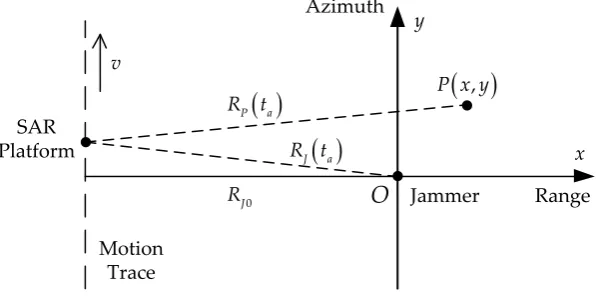
The JSF is the key to the generation of jamming signals. The following illustrates the basic idea for JSF in combination with the geometric model of SAR jamming. As shown in Figure 2, we assume that the SAR platform moves at a constant velocity 𝑣, and the azimuth time 𝑡𝑎= 0 when the plane
of zero Doppler passes through the jammer. A Cartesian coordinate system with the location of jammer as the origin is established in two-dimensional slant range plane. The x-axis points to the range direction and the y-axis points to the azimuth direction. The shortest slant distance between the jammer and the SAR is 𝑅𝐽0, and the instantaneous slant distance is 𝑅𝐽(𝑡𝑎) at azimuth time 𝑡𝑎.
An arbitrary false point scatter 𝑃 is generated by the jammer, the scattering coefficient of 𝑃 is 𝜎𝑃
and the location is (𝑥, 𝑦) in the coordinate above. 𝑅𝑃(𝑡𝑎) denotes the instantaneous slant distance
between 𝑃 and the jammer.
SAR Platform
Jammer
x y
v
Motion Trace
Range Azimuth
O
( )
P a
R t
( )
J a
R t
0 J R
( )
,P x y
Figure 2. The geometric model of SAR deceptive jamming.
𝐻𝑃(𝑓𝑟, 𝑡𝑎) = 𝜎𝑃exp [−𝑗2𝜋(𝑓𝑟+ 𝑓0)
2𝛥𝑅𝑃(𝑡𝑎)
𝑐 ] , (1)
where 𝑓𝑟 is the range frequency, 𝑐 is the velocity of light, Δ𝑅𝑃(𝑡𝑎) is the difference between 𝑅𝑃(𝑡𝑎)
and 𝑅𝐽(𝑡𝑎):
Δ𝑅𝑃(𝑡𝑎) = 𝑅𝑃(𝑡𝑎) − 𝑅𝐽(𝑡𝑎) = √(𝑥 + 𝑅𝐽0) 2
+ (𝑦 − 𝑣𝑡𝑎)2− √𝑅𝐽02 + (𝑣𝑡𝑎)2 . (2)
By calculating the JSF for each scatter in the template 𝑇, the JSF for the deception scene can be derived as follows:
𝐻(𝑓𝑟, 𝑡𝑎) = ∑ 𝐻𝑃(𝑓𝑟, 𝑡𝑎) 𝑃∈𝑇
= ∑ 𝜎𝑃exp [−𝑗2𝜋(𝑓𝑟+ 𝑓0)
2𝛥𝑅𝑃(𝑡𝑎)
𝑐 ]
𝑃∈𝑇
. (3)
In the implementation of jamming, the jammer must calculate JSF 𝐻(𝑓𝑟, 𝑡𝑎) and modulate the
intercepted signal real-time in each PRI. Because the calculation of equation (2) is time-consuming, the method represented by Equation (3) cannot be used directly for large scene deceptive jamming unless some improvements are made.
2.2 TDFS-TS Algorithm
2.2.1 Deceptive Jamming Based on TDFS
For space-borne SAR, we can assert that 𝑅𝐽0≫ 𝑥, 𝑅𝐽0≫ 𝑦 and 𝑅𝐽0≫ 𝑣𝑡𝑎 throughout the
synthetic aperture time. After the Taylor series expansion, Equation (2) can be approximated as follows [11]:
Δ𝑅𝑃(𝑡𝑎) ≈ [𝑥 + 𝑅𝐽0+
𝑦2
2(𝑥 + 𝑅𝐽0)
− 𝑦𝑣𝑡𝑎 𝑥 + 𝑅𝐽0
+ (𝑣𝑡𝑎)
2
2(𝑥 + 𝑅𝐽0)
] − [𝑅𝐽0+
(𝑣𝑡𝑎)2
2𝑅𝐽0 ] ≈ 𝑥 + 𝑦 2 2𝑅𝐽0 −𝑦𝑣𝑡𝑎 𝑅𝐽0 . (4)
With the approximation above, the JSF i.e. Equation (1) can be rewritten as follows: 𝐻𝑃(𝑓𝑟, 𝑡𝑎) = 𝜎𝑃exp [−𝑗2𝜋(𝑓𝑟+ 𝑓0) (
2𝑥 𝑐 +
𝑦2 𝑐𝑅𝐽0
−2𝑦𝑣𝑡𝑎 𝑐𝑅𝐽0
)]
= σPexp [−𝑗2𝜋(𝑓𝑟+ 𝑓0)
2𝑥
𝑐] exp (𝑗2𝜋𝑓0 2𝑦𝑣𝑡𝑎
𝑐𝑅𝐽0
) exp (−𝑗2𝜋𝑓0
𝑦2
𝑐𝑅𝐽0
)
exp (𝑗2𝜋𝑓𝑟
2𝑦𝑣𝑡𝑎− 𝑦2
𝑐𝑅𝐽0
) .
(5)
where the third exponential term is independent of 𝑓𝑟 and 𝑡𝑎 , it is equivalent to introduce a fixed
phase that has no effect on the imaging and can be ignored. The fourth exponential term can also be omitted when 𝑦 is small enough (details will be analyzed in the next subsection). So the Equation (5) can be simplified as follows:
𝐻𝑃(𝑓𝑟, 𝑡𝑎) = 𝜎𝑃exp [−𝑗2𝜋(𝑓𝑟+ 𝑓0)
2𝑥
𝑐] exp (𝑗2𝜋𝑓0 2𝑦𝑣𝑡𝑎
𝑐𝑅𝐽0
) . (6)
Actually, at the broadside mode, the azimuth frequency modulation rate of the SAR echo signal from the location of the jammer is [22]
𝐾𝑎= −
2𝑓0𝑣2
𝑐𝑅𝐽0
. (7)
Combined with Equation (6) and Equation (7), we can derive 𝐻𝑃(𝑓𝑟, 𝑡𝑎) = 𝜎𝑃exp [−𝑗2𝜋(𝑓𝑟+ 𝑓0)
2𝑥
𝑐] exp (−𝑗2𝜋𝐾𝑎 𝑦
It is equivalent to delaying the original echo signal 2𝑥/𝑐 in fast-time to achieve position deception in range dimension and shifting frequency −𝐾𝑎𝑦/𝑣 in slow-time. According to the frequency
shifting property of linear frequency modulation (LFM) signal, the frequency shifting is equivalent to time delaying 𝑦/𝑣 in slow-time, which can implement position deception in azimuth dimension as well.
If the scattering coefficient of the false point target which locates (𝑥, 𝑦) in the template is 𝜎(𝑥, 𝑦), the JSF for the deception scene can be derived as follows:
𝐻(𝑓𝑟, 𝑡𝑎) = ∑ ∑ 𝜎(𝑥, 𝑦) exp [−𝑗2𝜋(𝑓𝑟+ 𝑓0)
2𝑥
𝑐 ] exp (𝑗2𝜋𝑓0 2𝑦𝑣𝑡𝑎
𝑐𝑅𝐽0
)
𝑦 𝑥
= ∑ exp (𝑗4𝜋𝑓0
𝑦𝑣𝑡𝑎
𝑐𝑅𝐽0
)
𝑦
∑ 𝜎(𝑥, 𝑦) exp [−𝑗4𝜋(𝑓𝑟+ 𝑓0)
𝑥 𝑐]
𝑥
.
(9)
The second summation term in Equation (9) is independent with azimuth time 𝑡𝑎 and only related
to the relative position of each point in the false scene, which can be calculated off-line to reduce the real-time computational burden. This is the TDFS jamming algorithm, which has the advantages of simplicity and high computational efficiency.
2.2.2 Jamming Signal Analysis
Due to the approximation and simplification, the TDFS algorithm has high computational efficiency. However, the approximation and simplification will cause a decline in the image quality of the deceptive target at the same time. In this subsection, we will analyze the impact of the simplified operations above on the imaging results by comparing the difference between jamming signal and real point target echo in the range-Doppler domain [23].
The echo signal of a real scatter point 𝑃(𝑥, 𝑦) is represented as follows:
𝑠𝑃(𝑡𝑟, 𝑡𝑎) = 𝜎𝑃𝑤𝑎(𝑡𝑎)𝑤𝑟[𝑡𝑟−
2𝑅𝑃(𝑡𝑎)
𝑐 ] exp [−𝑗4𝜋𝑓0 𝑅𝑃(𝑡𝑎)
𝑐 ] exp {𝑗𝜋𝐾𝑟[𝑡𝑟−
2𝑅𝑃(𝑡𝑎)
𝑐 ]
2
} , (10)
where 𝑤𝑎(𝑡𝑎) represents azimuth amplitude, 𝑤𝑟(𝑡𝑟) is the SAR pulse complex envelop, and 𝐾𝑟 is
the frequency modulation rate of SAR pulse.
The parabolic approximation of instantaneous slant 𝑅𝑃(𝑡𝑎) by Taylor series is
𝑅𝑃(𝑡𝑎) = √(𝑥 + 𝑅𝐽0) 2
+ (𝑦 − 𝑣𝑡𝑎)2= 𝑥 + 𝑅𝐽0+
(𝑦 − 𝑣𝑡𝑎)2
2(𝑥 + 𝑅𝐽0)
. (11)
We can derive the echo signal expression (12) of real target point 𝑃(𝑥, 𝑦) in the range-Doppler domain by bring Equation (11) into Equation (10) and using the principle of stationary phase (POSP):
𝑆𝑃(𝑡𝑟, 𝑓𝑎) = 𝜎𝑃𝑊𝑎(𝑓𝑎)𝑤𝑟[𝑡𝑟−
2𝑅𝑃(𝑓𝑎)
𝑐 ]
exp {𝑗𝜋𝐾𝑟[𝑡𝑟−
2𝑅𝑃(𝑓𝑎)
𝑐 ]
2
− 𝑗𝜋𝑓𝑎
2
𝐾𝑎
− 𝑗2𝜋𝑓𝑎
𝑦
𝑣− 𝑗4𝜋𝑓0 𝑥 + 𝑅𝐽0
𝑐 } ,
(12)
where 𝑅𝑃(𝑓𝑎) is the range cell migration (RCM) curve of the target in the range-Doppler domain:
𝑅𝑃(𝑓𝑎) = 𝑥 + 𝑅𝐽0+
(𝑥 + 𝑅𝐽0)𝑐2
8𝑣2𝑓 02
𝑓𝑎2 , (13)
and the azimuth frequency modulation rate is
𝐾𝑎= −
2𝑣2𝑓 0
𝑐(𝑥 + 𝑅𝐽0)
. (14)
The echo signal will focus on the coordinate (𝑥, 𝑦) after range compression, RCM correction (RCMC) and azimuth compression.
𝑠𝐽(𝑡𝑟, 𝑡𝑎) = 𝜎𝑃𝑤𝑎(𝑡𝑎)𝑤𝑟[𝑡𝑟−
2𝑅𝐽(𝑡𝑎)
𝑐 −
2𝑥 𝑐]
exp {−𝑗4𝜋𝑓0[
𝑅𝐽(𝑡𝑎) 𝑐 + 𝑥 𝑐− 𝑦𝑣𝑡𝑎 𝑐𝑅𝐽0
]} exp {𝑗𝜋𝐾𝑟[𝑡𝑟−
2𝑅𝐽(𝑡𝑎)
𝑐 − 2𝑥 𝑐 ] 2 } . (15)
Similarly, the parabolic approximation and POSP is used to obtain the expression of jamming signal in the range-Doppler domain:
𝑆𝐽(𝑡𝑟, 𝑓𝑎) = 𝜎𝑃𝑊𝑎(𝑓𝑎)𝑤𝑟[𝑡𝑟−
2𝑅𝐽𝑃(𝑓𝑎)
𝑐 ]
exp {𝑗𝜋𝐾𝑟[𝑡𝑟−
2𝑅𝐽𝑃(𝑓𝑎)
𝑐 ]
2
− 𝑗𝜋𝑓𝑎
2
𝐾𝐽𝑎
− 𝑗2𝜋𝑓𝑎
𝑦
𝑣− 𝑗4𝜋𝑓0 𝑥 + 𝑅𝐽0
𝑐 + 𝑗2𝜋𝑓0 𝑦2
𝑐𝑅𝐽0
} , (16)
where the RCM of fake target is
𝑅𝐽𝑃(𝑓𝑎) = 𝑥 + 𝑅𝐽0+
𝑅𝐽0𝑐2
8𝑣2𝑓 02
𝑓𝑎2−
𝑦𝑐 2𝑣𝑓0
𝑓𝑎+
𝑦2
2𝑅𝐽0
, (17)
and the azimuth frequency modulate rate of jamming signal is
𝐾𝐽𝑎= −
2𝑣2𝑓 0
𝑐𝑅𝐽0
. (18)
It can be found that there are differences between the real target echo signal and the jamming signal in the RCM curve and azimuth frequency modulate rate with ignoring the phase term unrelated to pulse compression. The effects of these differences on the imaging results and the corresponding effective region of deceptive jamming are analyzed in detail below.
First, it is obvious that the jamming signal introduces the azimuth frequency modulate rate error, which will cause a mismatch of azimuth matched filter and lead to the main lobe broadening of the azimuth pulse compression result finally. The azimuth frequency modulate rate error is
Δ𝐾𝑎= 𝐾𝐽𝑎− 𝐾𝑎= −
2𝑣2𝑓 0𝑥
𝑐𝑅𝐽0(𝑥 + 𝑅𝐽0)
. (19)
The effect of Δ𝐾𝑎 on the main lobe broadening can be measured by the quadratic phase error
(QPE); the expression of QPE is as follows:
QPE = 𝜋Δ𝐾𝑎(
𝑇 2)
2
= − 2𝜋𝑣
2𝑓 0𝑥
𝑐𝑅𝐽0(𝑥 + 𝑅𝐽0)
(𝐿 2𝑣)
2
, (20)
where 𝑇 = 𝐿/𝑣 is the synthetic aperture time and 𝐿 represents the synthetic aperture length. For a typical Kaiser window with 𝛽 = 2.5, if the broadening is required to be less than 2%, 5%, and 10%, the corresponding QPE absolute value should be less than 0.27π, 0.41π and 0.55π [22]. Here we define the azimuth QPE factor 𝜀, when the condition |QPE| ≤ 𝜀𝜋 is required, the range coordinate 𝑥 should satisfy
|𝑥| ≤2𝜀𝑐𝑅𝐽0(𝑥 + 𝑅𝐽0) 𝑓0𝐿2
≈ 2𝜀 𝑐 𝑓0
(𝑅𝐽0 𝐿 )
2
. (21)
Second, in the range-Doppler domain, the RCM error of the jamming signal is
Δ𝑅𝑃(𝑓𝑎) = 𝑅𝐽𝑃(𝑓𝑎) − 𝑅𝑃(𝑓𝑎) = −
𝑥𝑐2
8𝑣2𝑓 02
𝑓𝑎2−
𝑦𝑐 2𝑣𝑓0
𝑓𝑎+
𝑦2
2𝑅𝐽0 . (22)
The last term in Equation (22) can be omitted because 𝑅𝐽0≫ 𝑦. The residual RCM introduced by
Δ𝑅𝑃(𝑓𝑎) in broadside mode is represented as follows:
RCMres= |Δ𝑅𝑃(
𝐵𝑎
2) − Δ𝑅𝑃(− 𝐵𝑎
2)| = 𝐵𝑎𝑐
2𝑣𝑓0
|𝑦| , (23)
𝐵𝑎=
𝐿 𝑣|𝐾𝐽𝑎| =
2𝑣𝑓0𝐿
𝑐𝑅𝐽0
. (24)
Combined with Equation (23) and Equation (24), we can simplify the expression of residual RCM: RCMres=
𝐿 𝑅𝐽0
|𝑦| . (25)
The residual RCM will result in the main lobe broadening in both range and azimuth dimension and the extent of broadening can be measured by the ratio of the residual RCM to the range resolution. The range resolution 𝜌𝑟≈ 𝑐/2𝐵, where 𝐵 is the signal bandwidth. Then define the residual RCM
factor 𝜂, if we require RCMres≤ 𝜂𝜌𝑟, the azimuth coordinate 𝑦 should satisfy
|𝑦| ≤ 𝜂𝜌𝑟𝑅𝐽0 𝐿 = 𝜂
𝑐𝑅𝐽0
2𝐵𝐿 . (26)
According to reference [22], the residual RCM should be no more than 0.5 range cell, therefore 𝜂 should be no more than 0.5.
In addition, due to the difference between the false and real point target in instantaneous slant range history, the Doppler center frequency of the jamming signal shifts, and the azimuth main lobe broadening and ghost targets are introduced. This phenomenon limits the effective azimuth scale as well, according to reference [11] the azimuth coordinate 𝑦 should satisfy
|𝑦| ≤𝑐𝑅𝐽0 2𝑣𝑓0
(PRF −𝑣 𝐷) −
𝐿
2 , (27)
where 𝐷 is the antenna aperture in azimuth.
Equation (21) and Equation (26) described the effective region on range and azimuth direction of the TDFS algorithm with the specified azimuth QPE factor 𝜀 and residual RCM factor 𝜂. The jamming signals representing the false target who locates beyond the region will not achieve the desired deception. Equation (27) described the inherent limitations of SAR deceptive jamming in azimuth direction which is beyond the scope of this article. In the following discussion, we suppose that the size of the template in the azimuth dimension meets the requirement of Equation (27). When a typical C-band space-Borne SAR parameters (see Table 1 in Section 3) are set as an example, we can calculate the effective region: |𝑥| ≤ 1.25 km and |𝑦| ≤ 0.75 km with ε = 0.25 and 𝜂 = 0.5, i.e. a rectangular area of 2.5 km × 1.5 km.
2.2.3 Template Segmentation
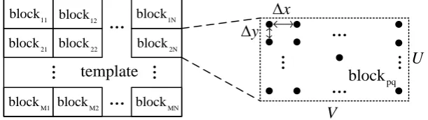
The analysis in the previous subsection shows that the effective region of the TDFS algorithm is limited. In order to achieve deceptive jamming in a larger scene, we divide the jamming scene template into several blocks and apply time-delay and frequency-shift in each block to calculate the partial JSF, which will be summed to get the JSF on the whole template. As shown in Figure 3, the template consisting of 𝑚 × 𝑛 point scatters is divided into 𝑀 × 𝑁 blocks, each block contains 𝑈 × 𝑉 point scatters, namely 𝑈 = 𝑚/𝑀 and 𝑉 = 𝑛/𝑁. If the range interval between each point is Δ𝑥 and the azimuth interval is Δ𝑦, 𝑈 and 𝑉 should satisfy the following conditions according to the limitation of the effective region Equation (21) and Equation (26) with the required 𝜀 and 𝜂:
𝑈 ≤ 𝜂𝑐𝑅𝑚𝑖𝑛
𝐵𝐿Δ𝑦, 𝑉 ≤ 4𝜀 𝑐 𝑓0Δ𝑥
(𝑅𝑚𝑖𝑛 𝐿 )
2
, (28)
where 𝑅𝑚𝑖𝑛 is the minimum value of the shortest slant range of all point scatters, which can be
…
…
…
…
template
…
…
…
…
x
y
11 block 12block block1N
21
block block22 block2N
M1
block blockM2 blockMN
U
V
pq
block
Figure 3. Jamming scene template segmentation diagram.
The scattering coefficients of point scatters in blockpq can be expressed as a matrix 𝐓𝑝𝑞:
𝐓𝑝𝑞= [
𝜎11 𝜎12 ⋯ 𝜎1𝑉
𝜎21 𝜎22 ⋯ 𝜎2𝑉
⋮ ⋮ ⋱ ⋮
𝜎𝑈1 𝜎𝑈2 ⋯ 𝜎𝑈𝑉
] . (29)
Suppose the coordinate of blockpq geometric center is (𝑥𝑞, 𝑦𝑝), where 𝑝 = 1, 2, ⋯ , 𝑀 and 𝑞 =
1, 2, ⋯ , 𝑁. According to Equation (1) and Equation (2), the JSF on blockpq geometry center
𝐻𝑐𝑝𝑞(𝑓𝑟, 𝑡𝑎) is represented as follows:
𝐻𝑐𝑝𝑞(𝑓𝑟, 𝑡𝑎) = exp {−
𝑗4𝜋(𝑓𝑟+ 𝑓0)
𝑐 [√(𝑥𝑞+ 𝑅𝐽0)
2
+ (𝑦𝑝− 𝑣𝑡𝑎) 2
− √𝑅𝐽02 + (𝑣𝑡𝑎)2]} . (30)
The jamming signal generated by 𝐻𝑐𝑝𝑞(𝑓𝑟, 𝑡𝑎) can generate a well-focused point target in the
center of blockpq after imaging processing, which is equivalent to moving the jammer to the location
of blockpq geometric center.
Then use the TDFS algorithm to generate the JSF on blockpq:
𝐻𝑝𝑞(𝑓𝑟, 𝑡𝑎) = 𝐻𝑐𝑝𝑞(𝑓𝑟, 𝑡𝑎) ∑ exp [
𝑗4𝜋𝑓0𝑣𝑡𝑎𝛥𝑦
𝑐(𝑅𝐽0+ 𝑥𝑞)
(𝑘 −𝑈 + 1 2 )]
𝑈
𝑘=1
∑ 𝜎𝑘𝑙exp [−
𝑗4𝜋(𝑓0+ 𝑓𝑟)𝛥𝑥
𝑐 (𝑙 −
𝑉 + 1 2 )]
𝑉
𝑙=1
,
(31)
where 𝜎𝑘𝑙 is the element of row 𝑘 and column 𝑙 in the matrix 𝐓𝑝𝑞. Finally, the JSF on the whole
template can be derived by summing JSF on all blocks:
𝐻(𝑓𝑟, 𝑡𝑎) = ∑ ∑ 𝐻𝑝𝑞(𝑓𝑟, 𝑡𝑎) 𝑁
𝑞=1 𝑀
𝑝=1
. (32)
Since the number of blocks is very small compared to the total number of scatters in the template, Equation (30) has a limited effect on the computing load. In addition, the second summation term of Equation (31) is independent of slow time 𝑡𝑎 and can be calculated offline. The template
segmentation method can solve the problem that the effective region of the TDFS algorithm is limited and achieve the purpose of the rapid generation of large scene deceptive jamming signals.
2.2.4 Correction Algorithm in Squint Mode
These analyses above are based on the broadside mode with the squint angle 𝜃 = 0. In order to extend the broadside jamming algorithm to squint mode, this subsection will discuss the effect of the squint angle on the jamming result and the corresponding correction method. It should be pointed out that the parabolic approximation of the instantaneous slant range in Equation (4) will no longer be applicable under the condition of large squint angle, so the jamming method of this article is limited to the small squint angle and the medium aperture length SAR.
First, the Doppler center frequency of the echo signal 𝑓𝑎𝑐= 2𝑣𝑓0sin 𝜃 /𝑐, the presence of the
position offset besides main lobe broadening in pulse compression [22]. According to the pulse compression principle, the azimuth main lobe position offset of scatter with coordinate (𝑥, 𝑦) is
𝑦𝑜𝑓𝑠(𝑥, 𝑦) = −
Δ𝐾𝑎
𝐾𝑎
𝑡𝑎𝑐𝑣 = 𝑥 tan 𝜃 , (33)
where 𝑡𝑎𝑐= −𝑅𝐽0tan 𝜃 /𝑣 is the pulse center time of the jamming signal in the azimuth dimension.
On the other hand, when 𝑓𝑎𝑐≠ 0, the RCM error will cause the RCM curve to shift along the
range dimension in addition to introducing the residual RCM to cause main lobe broadening. According to Equation (22), the offset on range dimension of fake point 𝑃(𝑥, 𝑦) is
𝑥𝑜𝑓𝑠(𝑥, 𝑦) = Δ𝑅𝑃(𝑓𝑎𝑐) ≈ −
𝑥 2sin
2𝜃 − 𝑦 sin 𝜃 . (34)
The residual RCM will increase at the same time: RCMres= |Δ𝑅𝑃(𝑓𝑎𝑐+
𝐵𝑎
2) − Δ𝑅𝑃(𝑓𝑎𝑐− 𝐵𝑎
2)| = | 𝐵𝑎𝑐
2𝑣𝑓0
𝑦 +𝐵𝑎𝑐 sin 𝜃 4𝑣𝑓0
𝑥| . (35)
In order to ensure the image quality of the fake scene, the size of the blocks should be reduced. However, the RCMres increment is not obvious when the squint angle is small. So it can be ignored
in this paper.
According to the analysis above, the main effect of the squint angle is the location offset of fake targets in the deceptive image, and the offset depends on the coordinates in the template. This effect will cause distortion of the jamming image. Therefore, the coordinates of each scatter in the template should be corrected. For the false scatter with coordinate (𝑥, 𝑦), the corrected coordinate (𝑥𝑐, 𝑦𝑐) can
be represented as follows:
{
𝑥𝑐 = 𝑥 − 𝑥𝑜𝑓𝑠(𝑥, 𝑦) = 𝑥 +
𝑥 2sin
2𝜃 + 𝑦 sin 𝜃 ,
𝑦𝑐 = 𝑦 − 𝑦𝑜𝑓𝑠(𝑥, 𝑦) = 𝑦 − 𝑥 tan 𝜃.
(36)
Correspondingly, Equation (31) will be modified as follows:
𝐻𝑝𝑞(𝑓𝑟, 𝑡𝑎) = 𝐻𝑐𝑝𝑞(𝑓𝑟, 𝑡𝑎) ∑ ∑ 𝜎𝑘𝑙 𝑉
𝑙=1 𝑈
𝑘=1
exp {−𝑗4𝜋(𝑓𝑟+ 𝑓0)Δ𝑥
𝑐 [(1 +
sin2𝜃
2 ) (𝑙 −
𝑉 + 1
2 )
+ Δ𝑦 sin 𝜃 (𝑘 −𝑈 + 1
2 )]} exp {
𝑗4𝜋𝑓0𝑣𝑡𝑎
𝑐(𝑅𝐽0+ 𝑥𝑞)
[−𝛥𝑥 tan 𝜃 (𝑙 −𝑉 + 1
2 ) + 𝛥𝑦 (𝑘 −
𝑈 + 1 2 )]} .
(37)
The range and azimuth related terms in Equation (37) are separable, so Equation (37) can be rewritten as matrix operations to increase the calculation speed. Here we define time-delay matrixes 𝐇𝐫1, 𝐇𝐫2 and frequency-shift matrixes 𝐇𝐚𝑞1, 𝐇𝐚𝑞2:
𝐇𝐫1=
[
exp [−𝑗4𝜋(𝑓𝑟+ 𝑓0)𝛥𝑥
𝑐 (1 +
sin2𝜃 2 ) (1 −
𝑉 + 1 2 )]
exp [−𝑗4𝜋(𝑓𝑟+ 𝑓0)𝛥𝑥
𝑐 (1 +
sin2𝜃
2 ) (2 − 𝑉 + 1
2 )] ⋮
exp [−𝑗4𝜋(𝑓𝑟+ 𝑓0)𝛥𝑥
𝑐 (1 +
sin2𝜃
2 ) (𝑉 − 𝑉 + 1
2 )]]
, (38)
𝐇𝐫2=
[
exp [−𝑗4𝜋(𝑓𝑟+ 𝑓0)𝛥𝑦 sin 𝜃
𝑐 (1 −
𝑈 + 1 2 )]
exp [−𝑗4𝜋(𝑓𝑟+ 𝑓0)𝛥𝑦 sin 𝜃
𝑐 (2 −
𝑈 + 1 2 )] ⋮
exp [−𝑗4𝜋(𝑓𝑟+ 𝑓0)𝛥𝑦 sin 𝜃
𝑐 (𝑈 −
𝑈 + 1 2 )]]
𝐇𝐚𝑞1=
[
exp [−𝑗4𝜋𝑓0𝑣𝑡𝑎𝛥𝑥 tan 𝜃 𝑐(𝑅𝐽0+ 𝑥𝑞)
(1 −𝑉 + 1 2 )]
exp [−𝑗4𝜋𝑓0𝑣𝑡𝑎𝛥𝑥 tan 𝜃 𝑐(𝑅𝐽0+ 𝑥𝑞)
(2 −𝑉 + 1 2 )] ⋮
exp [−𝑗4𝜋𝑓0𝑣𝑡𝑎𝛥𝑥 tan 𝜃 𝑐(𝑅𝐽0+ 𝑥𝑞)
(𝑉 −𝑉 + 1 2 )]]
, (40)
𝐇𝐚𝑞2=
[
exp [𝑗4𝜋𝑓0𝑣𝑡𝑎𝛥𝑦 𝑐(𝑅𝐽0+ 𝑥𝑞)
(1 −𝑈 + 1 2 )]
exp [𝑗4𝜋𝑓0𝑣𝑡𝑎𝛥𝑦 𝑐(𝑅𝐽0+ 𝑥𝑞)
(2 −𝑈 + 1 2 )] ⋮
exp [𝑗4𝜋𝑓0𝑣𝑡𝑎𝛥𝑦 𝑐(𝑅𝐽0+ 𝑥𝑞)
(𝑈 −𝑈 + 1 2 )]]
. (41)
Equation (37) is rewritten as follows:
𝐻𝑝𝑞(𝑓𝑟, 𝑡𝑎) = 𝐻𝑐𝑝𝑞(𝑓𝑟, 𝑡𝑎) [(𝐇𝐫2∘ 𝐇𝐚𝑞2) T
𝐓𝑝𝑞(𝐇𝐫1∘ 𝐇𝐚𝑞1)] , (42)
where (∙)T represents matrix transposition and the operator ∘ represents the Hadamard product of
matrix.
We can get the JSF of jammer on the entire scene by superimposing the JSF on all blocks, which is the same as Equation (32). The time-delay matrixes 𝐇𝐫1 and 𝐇𝐫2 are independent with azimuth
time 𝑡𝑎, which can be calculated offline in advance to improve real-time processing speed.
2.3 TDFS-TS Algorithm Procedure
The prerequisite for successful implementation of SAR deceptive jamming is to obtain relevant intelligence on the jamming object, which mainly include the follows aspects.
• Kinematic parameters of the SAR platform, including motion trajectory, motion velocity 𝑣, etc. The motion trajectory information is used to establish the jamming coordinate system and determine 𝑅𝐽0, the shortest distance between the jammer and SAR.
• Antenna parameters, including squint angle 𝜃, synthetic aperture length 𝐿, etc. • Signal parameters, including carrier frequency 𝑓0, bandwidth 𝐵, PRI, etc.
The specific detection methods of the parameters above will not be discussed in this paper; we just suppose that the parameters have been obtained in advance.
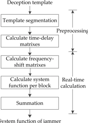
As shown in Figure 4, the entire procedure includes two parts, preprocessing and real-time calculation. The first step in the preprocessing stage is template segmentation, according to the parameters including synthetic aperture length 𝐿, signal bandwidth 𝐵, shortest slant range of the jammer 𝑅𝐽0 and the given factors 𝜀 and 𝜂, divide the template into several blocks based on the
limitation of Equation (28); then perform offline calculation and calculate the time-delay matrixes 𝐇𝐫1 and 𝐇𝐫2 according to Equation (38) and (39). In real-time calculation stage, calculate
frequency-shift matrixes 𝐇𝐚𝑞1, 𝐇𝐚𝑞2 according to Equation (40) and (41); then calculate JSF on each block based
Template segmentation
Calculate time-delay matrixes Deception template
Calculate frequency- shift matrixes
Calculate system function per block
Summation
System function of jammer
Preprocessing
Real-time calculation
Figure 4. TDFS-TS algorithm procedure.
3. Simulation Results
In this section, the effectiveness of the TDFS-TS algorithm is verified by simulating the imaging results of false point targets and fake scenes. The simulation results of the range dimension segmentation (RDS) algorithm proposed by Zhou et al. [11] are used as a comparison. The main parameters of radar which reference to the satellite RADARSAT-1 are listed in Table 1.
Table 1. The setting of SAR parameters in simulations.
Carrier
frequency Chirp rate PRF
Pulse width
Platform velocity
Shortest slant range
Antenna aperture
5.30 GHz 0.72
MHz/μs 1.26 kHz 41.74 μs 7.06 km/s 989 km 10 m
3.1 Fake Point Scatters Case
In order to analyze the imaging result of fake point scatter at different positions after imaging processing, a deceptive scene template containing only four-point scatters is set as shown in Figure 5. The four points 𝑃0∼ 𝑃3 are arranged in a rectangular shape with a distance of 6 km in range
dimension and 2 km in azimuth dimension. According to the calculation results in Subsection 2.2.2, set the length of blocks to 2.5 km in range dimension and 1.5 km in azimuth dimension. Since the imaging quality of fake scatters is only related to the position in the block, for the purpose of analyzing the jamming effect of the algorithm comprehensively, the template segmentation scheme is shown by the dashed line in Figure 5 so that 𝑃0 is located at the center of block, 𝑃1 is at the edge
of block in range dimension, 𝑃2 is at the azimuth edge, and 𝑃3 is at the edge of the block in both
range and azimuth dimension. In addition, the position of jammer (i.e. the origin position) is set at the point 𝑃0, actually the position of jammer has no effect on the imaging result. In the simulation of
0 1 2 3
-1 4
0 0.5 1.5
-0.5
Range(km)
A
zi
m
u
th
(k
m
)
0
P
P
12
P
P
31.0 2.0
5 6
Figure 5. The deceptive scene containing 4-point scatters.
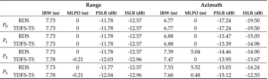
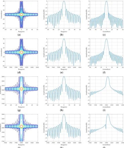
Figure 6 to Figure 9 show the imaging results of the four scatters by RDS and TDFS-TS algorithm in broadside mode and squint mode with the squint angle 𝜃 = 5°, including close-up image, range profile and azimuth profile. Table 2 and Table 3 list the imaging quality parameters of range and azimuth dimension in the two modes, including 3dB impulse response width (IRW), main lobe position offset (MLPO), peak sidelobe ratio (PSLR) and integrated sidelobe ratio (ISLR). It can be seen that compared with the RDS algorithm, the performance of TDFS-TS algorithm is basically equivalent, the RDS algorithm is more advantageous on IRW while TDFS-TS is dominant on MLPO. The IRW of TDFS-TS algorithm is increased especially for the azimuth dimension in squint mode, however the maximum broadening does not exceed 3.6%. In squint mode, the MLPO of RDS algorithm can reach up to -80.32 m in the azimuth dimension, which can be eliminated basically by TDFS-TS algorithm due to the corresponding correction. Because of the influence of residual RCM, the MLPO in the range dimension cannot be completely corrected, but the overall image is affected very little. In short, the simulation of fake point scatters shows that TDFS-TS algorithm is effective and has certain advantages in several areas.
Table 2. Comparison of imaging quality parameters between the RDS algorithm and TDFS-TS algorithm in broadside mode.
Range Azimuth
IRW (m) MLPO (m) PSLR (dB) ISLR (dB) IRW (m) MLPO (m) PSLR (dB) ISLR (dB)
𝑃0
RDS 7.73 0 -11.78 -12.57 6.77 0 -17.24 -19.50
TDFS-TS 7.73 0 -11.78 -12.57 6.77 0 -17.24 -19.50
𝑃1
RDS 7.73 0 -11.78 -12.57 6.88 0 -13.47 -15.05
TDFS-TS 7.73 0 -11.78 -12.57 6.88 0 -13.39 -14.98
𝑃2
RDS 7.73 0 -11.78 -12.57 7.39 5.04 -14.46 -14.90
TDFS-TS 7.78 -0.21 -12.03 -12.96 7.47 0 -13.95 -13.67
𝑃3
RDS 7.73 0 -11.77 -12.57 7.53 5.52 -15.03 -14.24
TDFS-TS 7.78 -0.21 -12.04 -12.96 7.60 0.48 -15.12 -12.55
Table 3. Comparison of imaging quality parameters between the RDS algorithm and TDFS-TS algorithm in squint mode with squint angle 𝜃 = 5°.
Range Azimuth
IRW (m) MLPO (m) PSLR (dB) ISLR (dB) IRW (m) MLPO (m) PSLR (dB) ISLR (dB)
𝑃0
RDS 7.73 0 -12.07 -12.79 6.77 0 -17.79 -20.30
TDFS-TS 7.73 0 -12.07 -12.79 6.77 0 -17.79 -20.30
𝑃1
RDS 7.88 -3.48 -12.79 -13.87 7.07 -80.32 -16.56 -17.91
TDFS-TS 7.88 7.69 -12.94 -13.92 7.15 -0.98 -18.76 -17.83
𝑃2
RDS 7.77 2.46 -12.02 -12.60 7.39 29.01 -15.03 -15.45
TDFS-TS 7.74 0.01 -11.68 -12.48 7.34 -0.01 -14.59 -14.96
𝑃3
RDS 7.95 -1.17 -12.36 -13.47 8.05 -50.70 -14.05 -14.08
(a) (b) (c)
(d) (e) (f)
(g) (h) (i)
(j) (k) (l)
(a) (b) (c)
(d) (e) (f)
(g) (h) (i)
(j) (k) (l)
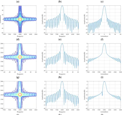
Figure 7. Simulation results of the TDFS-TS algorithm for false point scatters in broadside mode. Subfigures in each of the four rows (from up to down) are results of 𝑃0~𝑃3 respectively. Subfigures in each of the three columns (from left to right) are close-up radar image, range profile and azimuth profile, respectively.
(d) (e) (f)
(g) (h) (i)
(j) (k) (l)
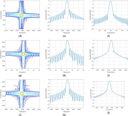
Figure 8. Simulation results of the RDS algorithm for false point scatters in squint mode with squint angle 𝜃 = 5°. Subfigures in each of the four rows (from up to down) are results of 𝑃0~𝑃3 respectively. Subfigures in each of the three columns (from left to right) are close-up radar image, range profile and azimuth profile, respectively.
(d) (e) (f)
(g) (h) (i)
(j) (k) (l)
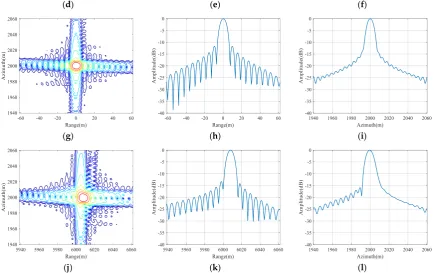
Figure 9. Simulation results of the TDFS-TS algorithm for false point scatters in squint mode with squint angle 𝜃 = 5°. Subfigures in each of the four rows (from up to down) are results of 𝑃0~𝑃3 respectively. Subfigures in each of the three columns (from left to right) are close-up radar image, range profile and azimuth profile, respectively.
3.2 General Deceptive Scene case
In this subsection, the TDFS-TS algorithm is applied to yield a fake scene. The jamming object is RADARSAT-1 whose parameters are listed in Table 1 and the squint angle 𝜃 ≈ −1.58°. The raw data of radar is obtained from the appendix of reference [22]. The fake scene template is another SAR image shown in Figure 10, whose length in the range dimension is 12.5 km and 4.5 km in the azimuth dimension. We divide the template according to the same block size calculated in subsection 2.2.2, as shown by the yellow line in Figure 10.
First, the signals generated by the two algorithms are processed to get the images which are shown in Figure 11 after amplitude normalized. Due to the existence of the squint angle, each segment of the image generated by the RDS algorithm has geometric distortion, which is especially obvious at the splicing of each segment. Moreover, since the positions of adjacent scatters in the template are shifted after the imaging process, the image is blurred and the brightness is weakened, and the ghost targets generated by the Doppler center frequency shifting in azimuth dimension will be more obvious after the amplitude normalization. These problems are solved by the TDFS-TS algorithm which corrected the geometric distortion caused by the squint angle.
Range
A
zi
m
u
th
A
zi
m
u
th
(a)
(b)
Figure 11. Imaging results of fake scene in Figure 10 using (a) RDS algorithm and (b) TDFS-TS algorithm.
(b)
(c)
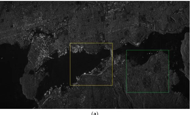
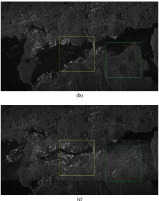
Figure 12. Comparison of jamming results. (a) is the image formed by the original signal. (b) is the image formed by the superposition of the original signal and jamming signal generated by the RDS algorithm. And (c) is the image formed by the superposition of the original signal and jamming signal generated by the TDFS-TS algorithm. Parts of the images marked by rectangular boxes will be enlarged and shown in Figure 13.
(d) (e) (f)
Figure 13. Partially enlarged image of Figure 12. Subfigures in each of the three columns (from left to right) are partially enlargement of the original image, the jamming image of the RDS algorithm and TDFS-TS algorithm. Subfigures in the first row are the enlarged images in yellow rectangular boxes and subfigures in the second row are in green boxes.
The imaging results of the superposition of the jamming signal and original signal are shown in Figure 12 and partially enlarged images are shown in Figure 13. It can be seen that the TDFS-TS algorithm achieves a good deception effect, generating clear false targets such as land and buildings and changing the topographic structure of the area protected. However, the fake scene generated by the RDS algorithm is not obvious mainly because of the decrease in brightness caused by geometric distortion. The jamming power has to increase in order to achieve a satisfactory jamming purpose, but the ghost targets will be strengthened at the same time. In conclusion, TDFS-TS algorithm has certain advantages compared with the RDS algorithm in large scene jamming.
4. Computational Complexity Analysis
The effectiveness of the TDFS-TS algorithm is verified by simulation in Section 3. In this section, we will estimate the computational complexity of the TDFS-TS algorithm to assess its practical value. Assume that the jamming scene template consists of 𝑚 × 𝑛 point scatters and is divided into 𝑀 × 𝑁 blocks, each block contains 𝑈 × 𝑉 point scatters. Here for ease of analysis, the addition, multiplication and power operations are all considered to be a basic operation. The following will analyze the number of basic operations to obtain the JSF 𝐻(𝑓𝑟, 𝑡𝑎) at a specific frequency 𝑓𝑟 and
azimuth time 𝑡𝑎.
In the preprocessing stage, calculating an element of matrix 𝐇𝐫1 requires 15 basic operations,
and the operation amount of all elements is 15𝑉, but because the elements in 𝐇𝐫1 are actually a
geometric series, other elements can be generated by multiplying the first element by the common ratio, so the amount of calculation is reduced to 15 + 𝑉. According to the same analysis, the operation amount of 𝐇𝐫2 is 12 + 𝑈, so the total computational complexity in the preprocessing stage is
𝐶𝑝𝑟𝑒= 15 + 𝑉 + 12 + 𝑈 = 𝑈 + 𝑉 + 27 . (43)
In the real-time calculation stage, calculating the JSF of a block center requires 20 basic operations, a total of 20𝑀𝑁 operations are required for all blocks. The operation amount for calculating matrix 𝐇𝐚𝑞1 is 15 + 𝑉, which needs to be repeated 𝑁 times. The calculation amount of matrix 𝐇𝐚𝑞2 is
14 + 𝑈, and needs to be repeated 𝑁 times as well. The computational complexity of matrix multiplication in Equation (42) is 2𝑈𝑉 + 𝑈 + 2𝑉 − 1, so the operation amount of Equation (42) is 2𝑈𝑉 + 𝑈 + 2𝑉 added the multiplication with 𝐻𝑐𝑝𝑞(𝑓𝑟, 𝑡𝑎), and the calculation of Equation (42) need
to be repeated 𝑀𝑁 times. Finally, the operation amount of the summation i.e. Equation (32) is 𝑀𝑁 − 1. Based on the analysis above, the total amount of computation in real-time calculation stage is
𝐶𝑟𝑡= 20𝑀𝑁 + 𝑁(15 + 𝑉) + 𝑁(14 + 𝑈) + 𝑀𝑁(2𝑈𝑉 + 𝑈 + 2𝑉) + 𝑀𝑁 − 1
= 𝑚𝑛 (2 +2 𝑈+
1 𝑉+
21
𝑈𝑉) + 𝑛 (1 + 𝑈 𝑉+
29 𝑉) − 1 .
According to the same analysis method, the computational complexity of different jamming algorithms including TDFS-TS, RDS, TDFS-TS without squint correction (TDFS-TS-WSC) and the basic algorithm (BA) shown by Equation (3) is derived and shown in Table 4.
Table 4. Computational complexity comparison of different algorithms
TDFS-TS RDS1 TDFS-TS-WSC BA
Preprocessing 𝑈 + 𝑉 + 27 𝑚𝑛 (14 −1
𝑉) 2𝑈𝑉 − 𝑈 + 𝑉 + 11 -
Real-time calculation
𝑚𝑛 (2 +2 𝑈+
1 𝑉+
21 𝑈𝑉) +𝑛 (1 +𝑈
𝑉+ 29
𝑉) − 1
22𝑚𝑛 𝑉 − 1
21𝑚𝑛 𝑈𝑉 +
𝑛
𝑉(3𝑈 + 13) − 1 21𝑚𝑛 − 1
1 the segment length in the range dimension of the RDS algorithm is the same as the block size of the TDFS-TS
algorithm.
(a) (b)
Figure 14. The relationship between the computational complexity and the total number of scatters in the template. (a) is the computational complexity in the preprocessing stage. (b) is the computational complexity in the real-time calculation stage.
The block size 𝑈 and 𝑉 are determined by the parameters of the jamming object, the scatter density of template, and the two imaging quality control factors 𝜀 and 𝜂. We fix 𝑈 and 𝑉 and observe the relationship between the computational complexity and the template size 𝑚 and 𝑛. According to the simulation parameters in Subsection 4.1, we set 𝑈 = 267 and 𝑉 = 539, draw the relationship between the computational complexity and the total number of scatters in the template shown in Figure 14. Here for the convenience of analysis, we set 𝑚 = 𝑛 and take the logarithm of computational amount for display.
algorithm is more efficient in the broadside mode, and the application scenario can be extended to the squint mode.
5. Conclusions
In this paper, the large scene electromagnetic deception of SAR is studied. The primary concern is to reduce the computation burden during the jamming process. For this purpose, the TDFS algorithm is proposed, which can improve the computation efficiency significantly. In addition, the focus capability of the jamming signal must be considered. In order to ensure the deceptive image quality of the TDFS algorithm in a large scene, the template is divided into several blocks according to the SAR parameters and imaging quality control factor. The correction algorithm in squint mode is introduced so that the TDFS-TS algorithm can be used to the SAR with a low squint angle and medium aperture length. Finally, simulation results and computational complexity analyses show that compared to other jamming algorithms the TDFS-TS algorithm has higher computational efficiency with less image quality decline in broadside mode. Furthermore, the application of parallel computation can partially compensate for the computational performance decline in squint mode.
The TDFS-TS algorithm is derived for space-borne SAR operating at broadside mode or low squint angle mode. In the future, we will investigate the rapid jamming method against the SAR with significant squint angle and long synthetic aperture. Additionally, other problems such as intelligence gathering and gain control, etc. will be studied as well.
Author Contributions: Conceptualization and supervision, W.Y.; formal analysis, F.M.; methodology, K.Y. and F.M.; experiment, G.L. and Q.T.; writing, K.Y.
Funding: This research was funded by Science and Technology on Complex Electronic System Simulation Laboratory, grant number DXZF-JC-ZZ-2017-007.
Conflicts of Interest: The authors declare no conflict of interest.
References
1. Walter, W.G. Synthetic Aperture Radar and Electronic Warfare; Artech House: Boston, MA, USA, 1993; pp. 25-39.
2. Condley, C.J. Some System Considerations for Electronic Countermeasures to Synthetic Aperture Radar. Proceedings of IEE Colloquium on Electronic Warfare Systems, London, UK, Jan. 1991; pp. 8/1-8/7. 3. Dumper, K.; Cooper, P.S.; Wons, A.F.; Condley, C.J.; Tully, P. Spaceborne Synthetic Aperture Radar and
Noise Jamming. Proceedings of the 1997 Radar Edinburgh International Conference, Edinburgh, UK, 14-16 Oct. 1997; pp. 411-414.
4. Fouts, D.J.; Pace, P.E.; Karow, C.; Ekestorm, S.R.T. A Single-Chirp False Target Radar Image Generator for Countering Wideband Imaging Radars. IEEE Journal of Solid-State Circuits2002, 37, 751-759.
5. Kristoffersen, S.; Thingsrud, O. The EKKO II Synthetic Target Generator for Imaging Radar. Proceedings of the 5th European conference on synthetic aperture radar, Ulm, Germany, May 2004; pp. 871-874. 6. Wei, Y.; Hang, R.; Shuxian, Z.; Li, Y. Study of Noise Jamming Based on Convolution Modulation to SAR.
Proceedings of 2010 International Conference on Computer, Mechatronics, Control and Electronic Engineering, Changchun, China, Aug. 2010, pp. 169-172.
7. Garmatyuk, D.S.; Narayanan, R.M. ECCM Capabilities of an Ultrawideband Bandlimited Random Noise Imaging Radar. IEEE Transactions on Aerospace and Electronic Systems2002, 28, 1243-1255.
8. Yan, Z.; Guoqing, Z.; Yu, Z. Research on SAR Jamming Technique Based on Man-made Map. Proceedings of International Conference on Radar, Shanghai, China, 16-19 Oct. 2006; pp. 1-4.
9. XiaoHong, L.; Peiguo, L.; Guoyi X. Fast Generation of SAR Deceptive Jamming Signal Based on Inverse Range Doppler Algorithm. Proceeding of IET International Radar Conference, Xi'an, China, 14-16 Apr. 2013; pp. 1-4.
10. Xiaodong, H.; Jun, Z.; Jun, W.; Dongping D.; Bin T. False Target Deception Jamming for Countering Missile-Borne SAR. Proceeding of IEEE 17th International Conference on Computational and Engineering, Chengdu, China, Dec. 2014; pp. 1974-1978.
12. Qingyang, S.; Ting, S.; Shicheng, Z.; Bin, T.; Wenxian, Y. A Novel Jamming Signal Generation Method for Deceptive SAR Jammer. Proceeding of 2014 IEEE Radar Conference, Cincinnati, USA, May 2014; pp. 1174-1178.
13. Bo, Z.; Feng, Z.; Zheng, B. Deception Jamming for Squint SAR Based on Multiple Receivers. IEEE Journal of Selected Topics in Applied Earth Observations and Remote Sensing2015, 8, 3988-3998.
14. Bo, Z.; Lei, H.; Feng, Z.; Jihong, Z. Performance Improvement of Deception Jamming Against SAR Based on Minimum Condition Number. IEEE Journal of Selected Topics in Applied Earth Observations and Remote Sensing2017, 10, 1039-1055.
15. Qingyang, S.; Ting, S.; Kaibor, Y.; Wenxian, Y.Efficient Deceptive Jamming Method of Static and Moving Targets Against SAR. IEEE Sensors Journal2018, 18; 3601-3618.
16. Yongcai, L.; Wei, W.; Xiaoyi, P.; Dahai, D.; Dejun, F. A Frequency-Domain Three-stage Algorithm for Active Deception Jamming Against Synthetic Aperture Radar. IET Radar, Sonar and Navigation2014, 8; 639-646. 17. Yongcai, L.; Wei, W.; Xiaoyi, P.; Qixiang, F.; Guoyu, W. Inverse Omega-K Algorithm for the
Electromagnetic Deception of Synthetic Aperture Radar. IEEE Journal of Selected Topics in Applied Earth Observations and Remote Sensing2016, 9; 3037-3049.
18. Bo, Z.; Lei, H.; Jian, L.; Maliang, L.; Jinwei, W. Deceptive SAR Jamming Based on 1-bit Sampling and Time-Varying Thresholds. IEEE Journal of Selected Topics in Applied Earth Observations and Remote Sensing2018, 11; 939-950.
19. Yongcai, L.; Wei, W.; Xiaoyi, P.; Letao, X.; Guoyu, W. Influence of Estimate Error of Radar Kinematic Parameter on Deception Jamming Against SAR. IEEE Sensors Journal2016, 16; 5904-5911.
20. Franceschetti, G.; Guida, R.; Iodice, A.; Riccio, D.; Ruello, G. Efficient Simulation of Hybrid Stripmap/Spotlight SAR Raw Signals From Extended Scenes. IEEE Transactions on Geoscience and Remote Sensing2004, 42; 2385-2396.
21. Ahmed, S.K.; Laurent, F.F.; Eric, P. Efficient SAR Raw Data Generation for Anisotropic Urban Scenes Based on Inverse Processing. IEEE Geoscience and Remote Sensing Letters2009, 6; 757-761.
22. Ian, G.C.; Frank, H.W. Digital Processing of Synthetic Aperture Radar Data: Algorithms and Implementation; Artech House: Boston, MA, USA, 2005; pp. 45-63.