A brief introduction to multivariate methods in grape and wine analysis

(1)

R E V I E W

A brief introduction to multivariate methods

in grape and wine analysis

D Cozzolino1 W U Cynkar1 N Shah1

R G Dambergs2 P A Smith1

1_{The Australian Wine Research}

Institute, Urrbrae, Glen Osmond, SA, Australia; 2_{The Australian Wine}

Research Institute, Tasmanian Institute of Agricultural Research, University of Tasmania, Hobart, Tasmania, Australia

Correspondence: Daniel Cozzolino The Australian Wine Research Institute. Waite Road, Urrbrae. PO Box 197, Glen Osmond SA 5064, Australia Fax: +61 8 8303 6601

Email [email protected]

Abstract: Real-world systems are usually multivariate and hence usually cannot be adequately described by one selected variable without the risk of serious misrepresentation. Analyzing the effect of one variable at a time by analysis of variance techniques can give useful descriptive information, but this will not give speciﬁ c information about relationships among variables and other important relationships in the entire matrix. Multivariate data analysis was developed in the late 1960s, and used by a number of research groups in analytical and physical organic chemistry due to the introduction of instrumentation giving multivariate responses for each sample analyzed. Development of such methods was also made possible by the availability of computers. Multivariate data analysis involves the use of mathematical and statistical techniques to extract information from complex data sets. The objective of this paper is to brieﬂ y describe and illustrate some multivariate data analysis methods used for grape and wine analysis.

Keywords: multivariate analysis, data mining, wine, grape

Introduction

Scientists in the food and beverage industry are faced with many different quality control tasks, including verifying that products meet required compositional and ﬂ avor standards, identifying changes in process parameters that might lead to a change in quality, detecting adulteration in raw materials and manufactured products, and identifying geographical origin of raw materials.1–3

Traditionally, much of the research in the ﬁ eld of grape and wine has been conducted in a manner that can be described as “univariate”, since it only examined the effect (response) of a single variable on the overall matrix.4–5_{Around the 1920s, when many} statistical methods were developed, samples were considered cheap and measurements expensive.6_{Since that time, the nature of technology has changed, samples are now} expensive (eg, the high cost of experiments) and measurements are cheap.

Analyzing the effect of one variable at a time by analysis of variance (ANOVA) techniques can give useful descriptive information, but this will not give speciﬁ c information about relationships among variables and other important relationships in the entire matrix.7–11_{Multivariate data analysis was developed in the late 1960s and} was used by a number of research groups in analytical and physical organic chemistry. Its development was due to the introduction of modern instrumentation, which gave multivariate responses for each sample analyzed (eg, wavelengths, ions, mass to charge ratios, chromatographic peaks) and to the wider availability of computers.9–13

In modern chemical measurements, we are often confronted with so much data that the essential information may be not readily evident.9–13_{Certainly that can be the case} with chromatographic or spectral data for which many different observations (peaks or wavelengths) have been collected from a single sample. Each different measurement can be thought of as a different dimension. Traditionally, analysts strive to eliminate matrix interference in analytical methods by isolating or extracting the analyte in

International Journal of Wine Research downloaded from https://www.dovepress.com/ by 118.70.13.36 on 23-Aug-2020

(2)

Cozzolino et al

order to make the measurement itself apparently simple and certain. However, this approach ignores the possible effects of chemical and physical interactions between the different constituents present in the sample, which is something that is especially evident when complex materials like grapes and wine are analysed.14–19

Univariate models do not consider the contributions of more than one variable source and can result in models that oversimplify the system under analysis. Therefore, in the modern scientiﬁ c approach, scientists need to look at the sample in its entirety and not just at a single component if we wish to untangle all the complicated interactions between the constituents and understand their combined effects on the whole matrix.20_{Multivariate methods provide the means} to move beyond the one-dimensional (univariate) world. In many cases, multivariate analysis can reveal constituents that are important through various interferences and interactions. This inductive rather than deductive reasoning needs a leap of imagination; it might be harder to accept and seemingly less certain and secure, but it opens a new chapter in the development of inferences from the analysis of the whole matrix.9–13,20_{Therefore, multivariate data analysis is deﬁ ned} as the application of mathematical or statistical methods to chemical data.

Multivariate data analysis, unlike classic statistics, considers multiple variables simultaneously. Although multivariate ANOVA (MANOVA) is available, other multivariate analytical methods have the advantage that they can take collinearity into account.7–8_{Multivariate analysis can} take into account the variation in one variable, or a group of variables, in terms of co-variation with other variables.8,20–22 The analysis can mathematically describe the co-variation (degree of association) between variables, or ﬁ nd a math-ematical function (regression model), by which the values of the dependent variables are calculated from values of the measured (independent) variables.20–22

Today, many food quality measurement techniques are multivariate and based on indirect measurements of chemical, physical, and sensory properties.5–8_{A typical characteristic} of many of the most useful of these instrumental techniques is that, paradoxically, the measurement variable might not have a direct relationship with the property of interest, for instance the concentration of a particular chemical in the sample, that is, a correlative method. This often refers to chemical and physical interference.20–22

Multivariate data analysis research spans a wide area of different methods which can be applied in different ﬁ elds of science and technology. They include methods

and techniques for collecting good data (optimization of experimental parameters, design of experiments, calibration, signal processing) and for getting information from these data (statistics, pattern recognition, modeling, structure– property–relationship estimations).8,11_{The most commonly} used multivariate data analysis techniques applied to grape and wine analysis are principal component analysis (PCA) and partial least squares (PLS) regression.9–13

The aim of this review is to give a brief description of different multivariate methods used in grape and wine analysis.

Brief description of multivariate

data methods

Both quantitative and qualitative applications of multivariate data analysis have been reported in the literature for the analysis of grape and wine. Most involve the use of PCA and PLS regression.14–19,23–43_{The following section describes} briefl y the different multivariate data analysis methods used. Many of the methods are based on the concept of soft modeling, a linear modeling method that originated in the fi eld of multivariate statistical analysis, but which has become synonymous with the term “chemometrics”. The focus of the soft modeling method on the properties of the signal, rather than on the noise, helps to distinguish multivariate data analysis from statistics, where the emphasis is usually on the structure and properties of the error term.9–13_Chemists often confuse the two fi elds, but remembering the difference in focus makes distinguishing them relatively simple.9–13

Because of the heavy emphasis on soft modeling in multivariate data analysis, the fi eld developed around an algorithmic rather than theoretical framework, an attribute that is now beginning to change.4,12–13,20–22_{Discussions of} soft modeling in current literature are more likely to focus on the linear algebraic theory of the modeling than on the specifi c steps needed to form the model.4,12–13,20–22_{It is useful} to have an appreciation for some of the key approaches and assumptions of soft modeling, as these underlie the logic of many of the multivariate analytical methods.10–13_For example modeling in spectroscopy has been done using “fi rst-principles” (hard) models. A hard model is one that describes the system in terms of a mathematical relationship developed using the measurement variables as independent variables and the desired outputs as dependent variables.7–8 Because chemical systems are generally complex, the hard modeling used in chemistry has either been applied to simpli-fi ed systems or has involved either limiting “laws” or other approximations and restrictions to the region of application

(3)

Multivariate methods in grape and wine analysis

of the hard model.7–8_{The ubiquitous “Beer’s Law” relations} used in quantitative spectroscopy is an example of one such ﬁ rst-principles model with well known limitations due to the simpliﬁ cations made in the theory.20–22

Soft modeling sees the modeling problem from an entirely different logical perspective. It assumes that the chemical system under study is complex and that it is not possible or economically feasible to adequately describe the behavior of the system using a hard model. The soft model is based on variation and correlation in the data, as captured in a covari-ance matrix, which can be thought of as a measure of the overall ﬂ uctuation in each independent variable present in the data set, as well as the variable–variable interactions.20–22

The ﬁ rst step in soft modeling is to express the data in terms of a new set of axes based on the different contribu-tions to variation in the data.7–8,20–22_{This is conveniently} done by a mathematical conversion from measured data to new axes based on covariance in the data set. A set of orthogonal components made from linear combinations of the independent (eg, spectral data) variables is created to describe independent sources of the observed variation in the covariance matrix created from the data set analyzed, according to the equation:

X = UVT

where matrix V, the loadings of the set of spectral data described by matrix X, contains the linear combinations of the original measurement variables that deﬁ ne the new variation-based coordinate system spanning the data in X and matrix U, called the scores of X, contains the coordinates of the data X in that variation-based coordinate system.20–22

The linear combinations of the measured spectral variables that result from the rotation are called latent variables because they are derived rather than measured. The latent variables extracted to describe a data set are ordered in terms of the size of the independent sources of variation that they explain. The ﬁ rst latent variable explains the largest independent source of variance in the data, the second latent variable the second largest, and so on, until all variation in the data set is accounted for by one of the linear combinations of the measurements.8,20–22

The second step in soft modeling is the elimination of noninformative latent variables. Generally, re-expression of the data set X in terms of latent variables is not useful unless a decision is also made on the number of latent variables that are needed to adequately explain the systematic varia-tion in the data X. At this point it is important to distinguish between the variables that help answer the questions posed

(and therefore must contain “signal”) and those that do not help (because they contain “noise”).8,20–22

Exploratory data analysis

Patterns of association exist in many data sets, but the relationships between samples can be difﬁ cult to discover when the data matrix exceeds three or more variables.20–22 Explor-atory data analysis can reveal hidden patterns in complex data by reducing the information to a more comprehensible form. Such multivariate data analysis can expose possible outliers and indicate whether there are patterns or trends in the data. Exploratory algorithms such as PCA and hierarchical cluster analysis (HCA) are designed to reduce large complex data sets into a series of optimized and interpretable views.8,13

Principal component analysis

PCA is used as a tool for screening, extracting, and compressing multivariate data.8,10–13_{PCA employs a} math-ematical procedure that transforms a set of possibly correlated response variables into a new set of noncorrelated variables called principal components.10–13_{PCA can be performed on} either a data matrix or a correlation matrix depending on the type of variables being measured. However, in a case where the original variables are nearly noncorrelated, noth-ing can be gained by usnoth-ing a PCA analysis. PCA produces linear combinations of variables that are useful descriptors or even predictors of some particular structure in the data matrix.8,11–13

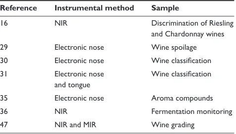
PCA is one of the most commonly used methods to analyze large data sets and has been applied to different types of instrumental methods as well as sensory data. For example, recent research has shown that rapid analysis of wine volatiles using an electronic nose (EN) instrument produces signals containing information that, even without chromatographic separation, can be used to determine a ﬁ ngerprint of wine based on its aroma proﬁ le.23–29_{The combination of PCA} analysis and gas sensors allow the detection of mass fragments formed during ionization of volatile compounds.23–29_This suggests that some of these volatiles are directly responsible for the sensory differences between samples and measuring the mass fragments of these compounds can provide some understanding of the chemical basis for sensory differentia-tion as well as a basis for varietal discriminadifferentia-tion.23–29_Other examples of the use of PCA applied to chemical, instrumental, and sensory data are shown in Table 1.

A combination of PCA and rapid methods is illustrated in Figure 1. The mid infrared (MIR) spectra (Figure 1A) of a set of wine samples (Shiraz, Riesling, and Sauvignon Blanc)

(4)

Cozzolino et al

and their principal component scores (Figure 1B) are plotted, indicating a separation between the wine samples analyzed. From the visual observation of the MIR spectra alone it is very hard to identify groups of samples related to variety. The use of PCA as a multivariate analytical tool allows the classiﬁ cation of wine samples according to variety (Shiraz, Riesling, and Sauvignon Blanc).

Discriminant analysis using PLS regression

Discriminant analysis (DA) can be considered a qualitative calibration method. Instead of calibrating for a con-tinuous variable, one calibrates for group membership (categories). In the case of two groups (eg, A and B) and several measurements there is a fairly obvious way to use regression methods to perform a DA. For example, create

an artiﬁ cial (dummy) Y-variable that has value 0 (zero) for each case in group A, and 1 (one) for each in group B, and develop a regression equation between Y and the X-variable measurements. The resulting models are evaluated in terms of their predictive ability to predict the Y variable of new and unknown samples (standard error of prediction, SEP). The use of DA and other classiﬁ cation tools can be found extensively in the analysis of grape and wine.14,29–31

Several studies have suggested that gas sensors together with DA methods might be used by the wine industry for the identiﬁ cation of white wine varieties or their blends.27–29_Even though the conventional analysis based on gas chromatography provides fundamental information about the volatile com-pounds present in the wine, the use of gas sensors has advan-tages of simplicity of sample preparation and reduced time of analysis.27–29_{For example, the use of EN was reported} to classify Riesling and unwooded Chardonnay wines from Australia and to discriminate between different wines, regions, vintages, and spoilage.29–32

In another study, metal oxide sensor (MOS) instruments were tested for the ability to characterize Ontario-produced fruit wines.33_{Eight fruit wines (blueberry, cherry, raspberry,} blackcurrant, elderberry, cranberry, apple, and peach) and four grape wines (red, Chardonnay, Riesling, and ice wines) were each obtained from ﬁ ve Ontario wineries. This study showed that it was possible to separate each wine variety based on differences between wineries.33_{The results show} that MOS instruments can discriminate between fruit and grape wines and may become an important tool for standard-ization of wine quality.33

Table 1 Use of principal component analysis and discriminant analysis combined with instrumental methods in the grape and wine industry

Reference Instrumental method Sample

16 NIR Discrimination of Riesling

and Chardonnay wines 29 Electronic nose Wine spoilage 30 Electronic nose Wine classifi cation 31 Electronic nose

and tongue

Wine classifi cation

35 Electronic nose Aroma compounds

36 NIR Fermentation monitoring

47 NIR and MIR Wine grading

Abbreviations: NIR, near infrared spectroscopy; MIR, mid infrared spectroscopy.

Wave numbers (cm–1₎

Absorbance

0.0

–0.10

–0.3 –0.2 –0.1 0.0 0.1 0.2 0.3 0.4 –0.05

0.00 0.05 0.10

0.2 0.4 0.6 0.8 1.0 1.2 1.4

PC1

PC2

RIES

RIES RIES RIES

RIES

SAUVB SAUVB

SAUVB SHSH

SH SH SHSH

SH

SH SH SH SH SH SH

RIES RIES

A B

Figure 1 A combination of PCA and rapid methods. A the mid-infrared spectra of a set of wine samples, B and their principal component scores.

Abbreviations: PCA,principal component analysis; PC, principal component score.

(5)

An application of EN (based on a tin oxide array) for the identifi cation of typical aromatic compounds present in white and red wines and responsible for different aroma attributes (eg, fruity, fl oral, herbaceous, vegetative, spicy, smoky) has also been reported.34,35_{Both PCA and DA showed that} datasets of these groups of compounds were clearly separated and confi rmed that the system could correctly discriminate the aromatic compounds added to the wine.34,35

Classi

fi

cation and clustering

Many applications require that samples be assigned to pre-defi ned categories, or “classes”. This may involve determining whether a sample is good or bad, or predicting an unknown sample as belonging to one of several distinct groups. A clas-sifi cation model is used to predict a sample class by comparing the sample to a previously analyzed experience set, in which categories are already known. Both k-nearest neighbour (KNN) and soft independent modeling of class analogy (SIMCA) are primary multivariate data analysis workhorses.11–13_{When these} techniques are combined to create a classifi cation model, the answers provided are more reliable and include the ability to reveal unusual samples or patterns in the data.11–13

Quantitative analysis: modeling

and calibration

In many applications, it is expensive, time consuming or difﬁ cult to measure a property of interest directly. Such cases require the analyst to predict the property of interest based on related properties that are easier to measure. The goal of multivariate data analysis regression analysis is to develop a calibration model which correlates the information in the set of known measurements to the desired property. Multivariate data analysis algorithms for performing regression include PLS and principal component regression (PCR) and are designed to avoid problems associated with noise and correla-tions in the data. Because the regression algorithms used are based on factor analysis, the entire group of known measure-ments is considered simultaneously, and information about correlations among the variables is automatically built into the calibration model. Multivariate data analysis regression lends itself handily to the on-line monitoring and process control industry, where fast and inexpensive systems are needed to test, predict, and make decisions about product quality.36

The modeling (regression) of one or several dependent Y-variables by means of a set of predictor responses (X-variables), is one of the most common applications of multivariate data analysis in science and technology. This is known as calibration and is one of the most important tasks

in quantitative analysis.4,8,9_{The principal aim is to} under-take regression analysis to develop a suitable mathematical model for descriptive or predictive purposes.12_{Examples of} mathematical models that help to deal with highly correlated data are PCR and PLS regression.4,8,9

Partial least squares regression

PLS regression is a recently developed generalization of multiple linear regression (MLR).4,8,9_{PLS regression is of} par-ticular interest because, unlike MLR, it can analyse data with strongly collinear (correlated), noisy and redundant variables (X variables) and can also model several characteristics (Y values) at the same time.4,8,9_{Note that the emphasis is on predicting the} characteristics and not necessarily on trying to understand the underlying relationships between the variables. PLS is a data reduction technique in that it reduces the X-variables to a set of noncorrelated factors that describe the variation in the data. However, if the number of factors used in the regression model is too large (greater than the number of samples) the models that fi t the sampled data perfectly might fail to predict new data.4,8,9_{This phenomenon is called overfi tting and is discussed} further below; as the number of factors is increased with a PLS calibration it approaches the model of multiple linear regression, which is notoriously prone to overfi tting when there is a large amount of X data relative to Y data to be predicted.4,8,9

A variant of PLS regression is locally weighted regression (LWR).37–40_{A potential problem with using the whole data} matrix is that large sample matrix variations within the dataset can create problems in developing a global PLS calibration, capable of predicting all samples.37–40_{This can} be a particular problem with agricultural products such as grape samples that can show seasonal variations and variations due to environmental effects. For example it has been demonstrated that seasonal and varietal variations can place constraints on calibration performance in the analysis of grapes with PLS regression of near infrared (NIR) spectra. When attempting to produce a universal calibration spanning many seasons, growing regions and grape varieties, the performance of PLS regression in prediction of grape anthocyanin was limited by pronounced nonlinearity.37–40 A potential method to minimize this matrix-related error is the use of “locally weighted” a regression algorithm that develops a PLS calibration from samples that best match the sample to be predicted. A particular software variant of LWR is the LOCAL algorithm, that uses a software driven selection process to match unknown samples with samples from a large calibration database, then uses a PLS calibration tailored to ﬁ t the unknown sample. It has been shown that

(6)

Cozzolino et al

LOCAL improves calibration performance over standard PLS, allowing universal application of calibrations for grape analytes across the wine industry, regardless of growing region, grape variety, and growing season.37–40

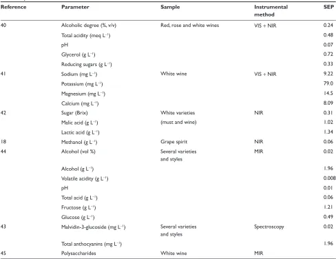
Table 2 summarizes some applications of PLS as a regression method to predict several compounds in grape, juice, and wine samples.

Arti

fi

cial neural networks

Application of artiﬁ cial neural networks (ANN) is a more recent technique for data and knowledge processing, char-acterized by its analogy with a biological neuron.10_When the ﬁ ring frequency of a neuron is compared with that of a computer, then for a neuron this frequency is rather low.10,51_{In the biological neuron the input signal from the} dendrites travels through the axons to the synapse. There

the information is transformed and sent across the synapse to the dendrites of the next neuron forming part of a highly complex network. The multivariate techniques based on ANN simulates the biological neuron by multiplication of the input signal (X) with the synaptic weight (W) to derive the output signal (Y).10,51_{Unlike linear regression, PCR and} PLS, ANN can deal with nonlinear relationships between variables. The performance of ANN is attributed to a high degree of interconnections. Like LOCAL regression, ANN can handle nonlinearity and outperforms standard PLS regression in that situation.34–36

Over

fi

tting and under

fi

tting

When using any of the data modeling techniques presented above, it is important to select an optimum number of variables or components.8_{If too many are used, too much}

Table 2 Use of partial least squares regression combined with instrumental methods to measure chemical compounds in grape and wine samples

Reference Parameter Sample Instrumental

method

SEP

40 Alcoholic degree (%, v/v) Red, rose and white wines VIS + NIR 0.24

Total acidity (meq L−1₎ _0.48

pH 0.07

Glycerol (g L−1₎ _0.72

Reducing sugars (g L−1₎ _0.33

41 Sodium (mg L−1₎ _{White wine} _VIS₊_NIR _9.22

Potassium (mg L−1₎ _79.0

Magnesium (mg L−1₎ _14.5

Calcium (mg L−1₎ _8.09

42 Sugar (Brix) White varieties NIR 0.31

Malic acid (g L−1₎ _{(must and wine)} _1.02

Lactic acid (g L−1₎ _1.34

18 Methanol (g L−1₎ _{Grape spirit} _NIR _0.06

44 Alcohol (vol %) Several varieties

and styles

MIR 0.02

Alcohol (g L−1₎ _1.96

Volatile acidity (g L−1₎ _0.008

pH 0.01

Total acid (g L−1₎ _0.06

Fructose (g L−1₎ _1.21

Glucose (g L−1₎ _0.49

43 Malvidin-3-glucoside (mg L−1₎ _{Several varieties}

and styles

Spectroscopy 0.02

Total anthocyanins (mg L−1₎ _1.96

45 Polysaccharides White wine MIR

Abbreviations: VIS + NIR, visible plus near infrared spectroscopy; MIR, mid infrared spectroscopy; SEP, standard error of prediction.

(7)

redundancy in the X-variables is modeled and the solution can become overfi tted; the model will be very dependent on the dataset and will give poor prediction results. On the other hand, using too few components will cause underfi tting and the model will not be large enough to capture the variability in the data. This “fi tting” effect is strongly dependent on the number of samples used to develop the model, and in general, more samples give rise to more accurate predictions.8

Conclusions

Multivariate data analytical methods both quantitative and qualitative are increasingly being used by research scientists in combination with traditional analytical tools. Multivariate data analysis techniques can be used to simplify methods and reduce analytical times for many compounds present in grapes and wine. Key factors contributing to the use of these methods in the grape and wine sector have been advances in instru-ment reliability, readily available multivariate data analysis software, and improved computing power. Compared to traditional methods, multivariate analysis combined with modern instrumental techniques (eg, EN, high-performance liquid chromatography, NIR and MIR spectrophotometers) often give new and better insight into complex problems by measuring a greater number of chemical compounds at once, thus enabling the “ﬁ ngerprinting” of each sample. These methods are attractive due to their inherent features of versa-tility, ﬂ exibility, effectiveness, and richness of information.

Acknowledgments

Comments and suggestions made by reviewers and editor in the original manuscript are acknowledged. This project is supported by Australia’s grapegrowers and winemakers through their investment body the Grape and Wine Research and Development Corporation, with matching funds from the Australian government. The work was conducted by The Australian Wine Research Institute.

References

1. Downey G. Authentication of food and food ingredients by near infrared spectroscopy. J Near Infrared Spec. 1996;4:47–61.

2. Downey G. Food and food ingredient authentication by mid-infrared spectroscopy and chemometrics. Trends Anal Chem. 1998;17: 418–424.

3. Arhurst PR, Dennis MJ. Food Authentication. London, UK: Blackie Academic and Professional; 1996.

4. Munck L, Norgaard L, Engelsen SB, Bro R, Andersson CA. Chemometrics in food science: a demonstration of the feasibility of a highly exploratory, inductive evaluation strategy of fundamental scientiﬁ c signiﬁ cance. Chem Intell Lab Sys. 1998;44:31–60. 5. Francis IL, Høj PB, Dambergs RG, et al. In: Blair R, Williams P,

Pretorious IS, editors. Proceedings 12th Australian Wine Industry Technical Conference. Adelaide, Australia: Winetitles; 2005.

6. Bendell A, Disney J, McCollin C. The future role of statistics in quality engineering and management. The Statistician. 1999;48:299–326. 7. Martens H, Martens M. Multivariate Analysis of Quality. An

Introduction. Hoboken, NJ: John Wiley and Sons, Ltd; 2000. 8. Naes T, Isaksson T, Fearn T, Davies T. A User-friendly guide to

multivariate calibration and classiﬁ cation. Chichester, UK: NIR Publications; 2002.

9. Wold S, Sjöstrom M, Eriksson L. PLS-regression: a basic tool of chemometrics. Chem Intell Lab Sys. 2001;58:109–130.

10. Otto M. Chemometrics: Statistics and computer application in analytical chemistry. Hoboken, NJ; Wiley-VCH; 1999.

11. Siebert KJ. Chemometrics in brewing: a review. J Amer Soc Brew Chem. 2001;59:147–156.

12. Adams MJ. Chemometrics in analytical spectroscopy(RSC Spectroscopy Monographs). London, UK: The Royal Society of Chemistry; 1995. 13. Brereton RG. Introduction to multivariate calibration in analytical

chemistry. The Analyst. 2000;125:2125–2154.

14. Arvantoyannis I, Katsota MN, Psarra P, Souﬂ eros E, Kallinthraka S. Application of quality control methods for assessing wine authenticity: Use of multivariate analysis (chemometrics). Trends Food Sci Technol. 1999;10:321–336.

15. Cordella Ch, Moussa I, Martel A-C, Sbirrazzuoli N, Lizzani-Cuvelier L. Recent developments in food characterisation and adulteration detec-tion: technique-oriented perspectives. J Agric Food Chem. 2000;50: 1751–1764.

16. Cozzolino D, Smyth HE, Gishen M. Feasibility study on the use of visible and near infrared spectroscopy to discriminate between white wine of different varietal origin. J Agric Food Chem. 2003;54: 7703–7708.

17. Cozzolino D, Kwiatkowski MY, Parker M, et al. Prediction of phenolic compounds in red wine fermentations by visible and near infrared spectroscopy. Anal Chim Acta. 2003;513:73–80.

18. Dambergs RG, Kambouris A, Francis IL, Gishen M. Rapid analysis of methanol in grape-derived distillation products using near infrared transmission spectroscopy. J Agric Food Chem. 2002;50:3079–3084. 19. Dambergs RG, Esler MB, Gishen M. Application in analysis of bever-ages and brewing products. In: Roberts CA, Workman J, Reeves JB, editors. Near Infrared Spectroscopy in Agriculture. Madison: Agronomy Monograph; 2004.

20. Geladi P. Chemometrics in spectroscopy. Part I. Classical chemometrics.

Spectrochimica Acta Part B. 2003;58:767–782.

21. Wold S. Chemometrics; what do we mean with it, and what do we want from it? Chem Intell Lab Sys. 1995;30:109–115.

22. Wise BM, Gallagher NB. The process chemometrics approach to process monitoring and fault detection. J Proc Cont. 1996;6:329–348. 23. Di Natale C, Davide FAM, D’Amico A, et al. Complex chemical pattern

recognition with sensor array: the discrimination of vintage years of wine. Sensor Actuat. 1995;25:801–804.

24. Di Natale C, Paolesse R, Burgio M, Martinelli E, Pennazza G, D’Amico A. Application of metalloporphyrins-based gas and liquid sensor arrays to the analysis of red wine. Anal Chim Acta. 2004;513:49–56.

25. Di Natale C, Paolesse R, Macagnano A, et al. Application of a combined artiﬁ cial olfaction and taste system to the quantiﬁ cation of relevant compounds in red wine. Sensor Actuat. 2000;69:342–347

26. Gutierrez A, Burgos JA, Garcera C, Padilla AI, Zarzo M, Chirivella C, Ruiz M L, Molto E. Optimization of an aroma sensor for assessing grape quality for wine making. Spanish J Agric Res. 2007;5:157–163. 27. Deisingh AK, Stone DC, Thompson M. Applications of electronic noses

and tongues in food analysis. Int J Food Sci Tech. 2004;39:587–604. 28. Cozzolino D, Smyth HE, Lattey KA, et al. Combining mass

spec-trometry based electronic nose, visible-near infrared spectroscopy and chemometrics to assess the sensory properties of Australian Riesling wines. Anal Chim Acta. 2006;563:319–324.

29. Cynkar WU, Cozzolino D, Dambergs RG, Janik L, Gishen M. Feasibility study on the use of a head space mass spectrometry electronic nose (MS e-nose) to monitor red wine spoilage induced by Brettanomyces yeast. Sensor Actuat. 2007;124:167–171.

(8)

Cozzolino et al

30. Aleixandre M, Lozano J, Gutierrez J, Sayago I, Fernandez MJ, Horrillo MC. Portable e-nose to classify different kinds of wine. Sensors and Actuators. 2008;131:71–76.

31. Buratti S, Bendetti S, Scampicchio M, Pangerod EC. Characterization and classiﬁ cation of Italian Barbera wines by using an electronic nose and an amperometric electronic tongue. Anal Chim Acta. 2004;525: 133–139.

32. Penza M, Cassano G. Chemometric characterization of Italian wines by thin-ﬁ lm multisensors array and artiﬁ cial neural networks. Food Chem. 2004;86:283–296.

33. McKellar RC, Vasantha-Rupasinghe HP, Xuewen L, Knight KP. The electronic nose as a tool for the classiﬁ cation of fruit and grape wines from different Ontario wineries. J Sci Food Agric. 2005;85:2391–2396. 34. Lozano J, Santos JP, Aleixandre M, Sayago I, Gutierrez J, Horrillo MC.

Identiﬁ cation of typical wine aromas by means of electronic nose. IEEE Sensors J. 2006;6:173–178.

35. Lozano J, Santos JP, Horrillo MC. Classiﬁ cation of white wine aromas with an electronic nose. Talanta. 2005;67:610–617.

36. Cozzolino D, Parker M, Dambergs RG, Herderich M, Gishen M. Chemometrics and visible-near infrared spectroscopic monitoring of red wine fermentation in a pilot scale. Biotech Bioeng. 2006;95: 1101–1107.

37. Esler MB, Gishen M, Francis IL, et al. Effects of variety and region on new infrared reﬂ ectance spectroscopic analysis of quality parameters in red wine grapes. In: Cho RK, Davies AMC, editors.

Proceedings of the 10th International Conference. Chichester, UK: NIR Publications; 2002.

38. Shenk JS, Berzaghi P, Westerhaus MO. Investigation of a LOCAL calibration procedure for near infrared instruments. J Near Infrared Spec. 1997;5:223–226.

39. Dambergs RG, Cozzolino D, Cynkar WU, Janik L, Gishen M. The determination of red-grape quality parameters using the LOCAL algorithm. J Near Infrared Spec. 2006;14:71–79.

40. Urbano-Cuadrado M, Luque de Castro MD, Perez-Juan PM, Garcia-Olmo J, Gomez-Nieto MA. Near infrared reflectance, spectroscopy and multivariate analysis in enology – Determination or screening of ﬁ fteen parameters in different types of wines. Anal Chim Acta. 2004;527:81–88.

41. Sauvage L, Frank D, Stearne J, Milikan MB. Trace metal studies of selected white wines and alternative approach. Anal Chim Acta. 2002;458:223–230.

42. Manley M, van Zyl A, Wolf EEH. The evaluation of the applicability of Fourier transform near-infrared (FT-NIR) sppectroscopy in the measurement of analytical parameters in must and wine. S A J Oenol Viti. 2001;22:93–100.

43. Soriano PM, Pérez-Juan A, Vicario JM, González Pérez-Coello MS. Determination of anthocyanins in red wine using a newly developed method based on Fourier transform infrared spectroscopy. Food Chem. 2007;104:1295–1303.

44. Patz C-D, Blieke A, Ristow R, Dietrich H. Application of FT-MIR spectrometry in wine analysis. Anal Chim Acta. 2004;513:81–89. 45. Coimbra MA, Goncalves F, Barros AS, Delgadillo I. Fourier transform

infrared spectroscopy and chemometric analysis of white wine polysac-charide extracts. J Agric Food Chem. 2002;50:3405–3411.

46. Lletí R, Meléndez E, Ortiz MC, Sarabia LA, Sánchez MS. Outliers in partial least squares regression: Application to calibration of wine grade with mean infrared data. Anal Chim Acta. 2005;544:60–70.

47. Nieuwoudt HH, Prior BA, Pretorius IS, Manley M, Bauer FF. Principal component analysis applied to Fourier transform infrared spectroscopy for the design of calibration sets for glycerol prediction models in wine and for the detection and classiﬁ cation of outlier samples. J Agric Food Chem. 2004;52:3726–3735.

48. Cozzolino D, Cynkar W, Janik L, Dambergs RG, Gishen M. Analysis of grape and wine by near infrared spectroscopy – a review. J Near Infrared Spectros. 2006;14:279–289.

49. Dixit V, Tewari JC, Cho B K, Irudayraj JMK. Identifi cation and quantifi cation of industrial grade glycerol adulteration in red wine with Fourier transform infrared spectroscopy using chemometrics and artifi cial neural networks. Appl Spectros. 2005;59:1553–1561. 50. Le Moigne M, Maury Ch, Bertrand D, Jourjon F. Sensory and

instru-mental characterisation of Cabernet Franc grapes according to ripening stages and growing location. Food Qual Pref. 2008;19:220–231. 51. Janik L, Cynkar WU, Cozzolino D, Dambergs RG, Gishen M. The

prediction of total anthocyanin concentration in red-grape homogenates using near-infrared spectroscopy and artiﬁ cial neural networks. Anal Chim Acta. 2007;594:107–118.