Continuum radiative transfer
Christophe Pinte1,2
1UMI-FCA, CNRS/INSU, France (UMI 3386), and Dept. de Astronomía, Universidad de Chile, Santiago,
Chile
2Univ. Grenoble Alpes, IPAG, F-38000 Grenoble, France
CNRS, IPAG, F-38000 Grenoble, France
Abstract.Understanding the properties and evolutionary stage of protoplanetary disks re-quires to be able to derive physical quantities from multi-wavelength and multi-technique observations of these disks. Because of the complexity of the radiative transfer, we must rely on sophisticated numerical codes to do so. In this chapter, we present the radiative transfer problem in dusty media and discuss why this represents a difficult numerical problem to solve. We briefly describe the various methods that can be used to solve the radiative transfer equation and discuss their relative merits and drawbacks.
1 Introduction
Dust grains represent only a small fraction of the mass of protoplanetary disks, of the order of 1 %. But they play a central role in the disk thermal structure because as they completely dominate the continuum opacities. At short wavelengths, dust grains efficiently absorb, scatter, and polarise the starlight while at longer wavelengths dust re-emits the absorbed radiation. How much radiation is scattered and absorbed is a function of both the geometry of the circumstellar environment and the properties of the dust. In turn, the amount of absorbed radiation sets the temperature of the dust (and gas) and defines the amount of radiation that is re-emitted at longer, thermal wavelengths.
With the advent of high-angular resolution and high-contrast instruments, the basic structural properties (e.g., size, inclination, and surface brightness) of the circumstellar environments of the nearest and/or largest objects — disks and envelopes around young stars in nearby star-forming re-gions and around more distant evolved stars — are now under close scrutiny. With this unprecedented wealth of high-resolution data, from optical to radio, detailed studies of the dust content become possible and sophisticated radiative transfer (RT) codes are needed to fully exploit the data.
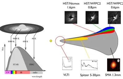
Because circumstellar disks remain optically thick over a broad wavelength range, a given ob-servation only probes a very limited part of the disk. Figure 1 illustrates the various regions of a protoplanetary disk probed using different observational techniques. To obtain a global picture of disks, it is critical to combine all these observations and to model them simultaneously.
5thLecture from Summer School “Protoplanetary Disks: Theory and Modelling Meet Observations” DOI: 10.1051/
C
Owned by the authors, published by EDP Sciences, 2015 /201
epjconf 51020 0 00
7KLVLVDQ2SHQ$FFHVVDUWLFOHGLVWULEXWHGXQGHUWKHWHUPVRIWKH&UHDWLYH&RPPRQV$WWULEXWLRQ/LFHQVHZKLFKSHUPLWV XQUHVWULFWHGXVHGLVWULEXWLRQDQGUHSURGXFWLRQLQDQ\PHGLXPSURYLGHGWKHRULJLQDOZRUNLVSURSHUO\FLWHG
8000 K 4000 K
400 K 40 K
DIS& 67$5
UV IR radio
flux
ZDYHOHQJWK
HST/Nicmos 1.6µm
HST/WFPC2 0.8µm
HST/WFPC2 0.6µm
VLTI Spitzer 5-30µm SMA 1.3mm
Figure 1. Left: origin of emission in the disk as a function of wavelength (Figure from R. Lachaume). Right: Schematic view of the complementarity between observations at various wavelengths. Various observing tech-niques allow probing distinct parts of the disk. In anti clock-wise direction from top right: scattered light images probe the disk surface, going deeper as the wavelength increases, PAHs’ emission probes a very superficial layer excited by stellar UV photons, near-IR interferometry probes the very central parts of the disk, mid-IR spec-troscopy allows studying the properties of the grains up to a few 10s of AUs, and observations at millimeter wavelengths allow probing the bulk of the disk mass.
2 Observables and radiative quantities
For an astronomer looking at a source through a telescope, there are 4 observables for radiation: energy flux, direction, frequency or wavelength and the polarization.
2.1 Radiative flux
Theradiative fluxis defined as the energy going through an elemental surface per units of time per unit of surface area. In CGS units this has the dimension of erg s−1cm−2.
F= dE
dAdt (1)
The fluxF is called the bolometric flux, but most of the time we are interested in measuring the flux in a specific wavelength or frequency range, and we can defined a monochromatic fluxFλorFν. The bolometric and monochromatic fluxes are related by
F=
∞
0
Fλdλ=
∞
0
Note that because dλ/ν=−λ/dν,FλFνbutλFλ=νFν. Several units are used in astronomy for the flux. In particular, it is often defined in Jansky, where 1 Jy=10−23erg s−1cm−2Hz−1. Note also that the flux is a vectorial quantity. The fluxFwe have defined is the component of the flux vector→−F that is perpendicular to dA:F=→−F.→−n where→−n is a unitary vector normal to dA.
2.2 Specific intensity
The flux is a measure of the energy carried by all the photons,i.e.from all directions, passing through a surface. In radiative transfer theory, we generally work with a connected quantity, thespecific inten-sity, which describes the amount of energy carried in a given direction. To define the specific intensity accurately in a given direction, we construct an infinitesimal area dAnormal to the chosen direction and we consider all the rays whose direction is within a solid angle dΩof the chosen direction. The energy crossing dA, in a time interval dtand a frequency range dνis given by
dE=IνdAdtdΩdν (3)
whereIνis the specific intensity.Iνis a 6 dimension quantity, it depends on the frequency, the 3 spatial dimensions and 2 angular directions. It has units of erg s−1cm−2Hz−1ster−1.
The specific intensity is connected to the flux by the following relation:
−→ Fν=
ΩIν( −
→n)→−ndΩ (4)
Note that ifIνis isotropic, the corresponding net flux is zero.
2.3 Moments of specific intensity
Because the specific intensity contains an extremely rich information, it is often sufficient to work with quantities that are angularly averaged. In particular, it is convenient to define the zeroth, first and second tensor moment of the radiation field:
Jν= 1 4π
ΩIν( −
→n) dΩ (5)
−→ Hν= 1
4π
ΩIν( −
→n) cosθ→−ndΩ (6)
Kν= 1 4π
ΩIν( −
→n) cos2θdΩ (7)
The zeroth moment Jνis called themean intensityand is the angular average of Iν. This quantity is of particular interest as it determines the heating (of dust and gas), the ionization and population levels. The first moment is proportional to the flux and describes the net flux of energy, while the second moment describes the radiation pressure.
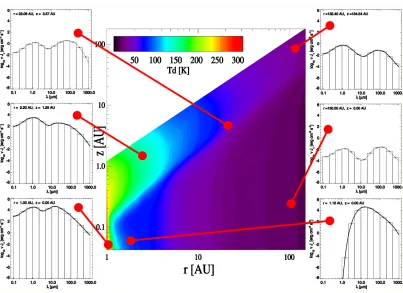
Figure 2.Shape of the radiation fieldJνas a function of the position in the disk. The central plot shows the dust
temperature structure of a typical disk surrounding a T Tauri star. Left column: the radiation field is dominated by the stellar radiation in the central parts, with a thermal component at longer wavelengths. At a few AUs in the midplane, the stellar radiation is completely attenuated and only the thermal emission remains (bottom right). At large distances, the radiation field is dominated by the diluted stellar light+thermal emission of the disk (top right), or the scattered light+thermal emission (middle right). Figure kindly provided by P. Woitke.
3 Radiative transfer
3.1 Specific intensity is constant along a ray in free space
One of the fundamental properties of the specific intensity is that, if we are following a ray in free space (i.e.vacuum), the intensity in the direction of the ray remains constant along that ray:
dIν
ds =0 (8)
where dsis a differential element of length along the ray.
3.2 Absorption and emission
When a ray passes through matter, energy can be added or removed and the specific intensity will not remain constant along the ray.
The energy emitted by a volume dV is defined by the spontaneous emission coefficient or emis-sivityjν:
dE= jνdVdΩdtdν (9)
wherejνhas dimension of erg s−1cm−3Hz−1ster−1.
When moving a distance ds, a beam of cross section dAtravels through a volume dV=dsdAand the intensity added to the beam is then:
dIν= jνds (10)
The loss of energy in a beam traveling a distance dsis described by
dIν=−ανIνds (11)
whereανis called the extinction coefficient and has units of cm−1. Eq. 11 means that the intensity along a ray decreases as the exponential of the absorption coefficient integrated along the line of sight:
Iν(s)=Iν(s0) exp
−
s
s0
αν(s) ds
(12)
This equation can easily understood if you consider a simple model of randomly distributed par-ticles with a particle densityn, each of the particles having a cross sectionσν(in cm2). If you now
consider a beam of radiation of surface dAalong a distance ds, the number of absorbing particles seen by the beam isndAds. The energy absorbed by the particles is:
dE=−dIνdAdΩdtdν=Iν(nσνdAds) dΩdtdν (13)
and then
dIν=−nσνIνds (14)
with
αν=nσν (15)
The opacity can also be defined per unit of mass: κν =αν/ρ(in cm2g−1), where ρis the local
density in g cm−3. Note that depending ifρis the gas or dust density, the opacity will be defined per
gram of gas or per gram of dust.
The optical depth between 2 pointss1ands2can be defined as:
τν(s1,s2)=
s2
s1
αν(s) ds (16)
The extinction coefficient is connected to the photon mean free path,i.e. the mean distance a photon can travel through a medium before being absorbed or scattered. The mean optical depth is given by
τν=
∞
0
τνe−τνdτν=1 (17)
Withτν=ανlν=1, we find that the mean free path islν=1/αν.
3.3 The radiative transfer equation and its formal solution
If we include the effects of emission and absorption in the differential equation for the specific intensity along a ray, we obtain :
dIν(s)
ds = jν(s)−αν(s)Iν(s) (18)
This equation can be formally integrated between 2 pointss1ands2giving:
Iν(s2)=Iν(s1)e−τν(s1,s2)+
s2
s1
jν(s)e−τν(s,s2)ds (19)
3.4 Kirchhoff’s law
Suppose you have a cavity filled with an emitting material of temperatureT, in thermal equilibrium with the cavity. Then, the intensity should be everywhereIν=Bν(T). If we write the radiative transfer equation, we obtain
dIν
ds = jν(s)−αν(s)Iν(s)= jν(s)−αν(s)Bν(T)=0 (20) and then
jν=ανBν(T) (21)
This relation is calledKirchhoff’s law. It means that the emissivity of a medium in thermal equi-librium is defined only by its temperature and the absorption coefficientαν. It applies everywhere the medium is in local thermodynamic equilibrium (LTE).
3.5 Source function
As a generalization of Kirchhoff’s law, we can define thesource function Sνas the ratio of the emis-sivity by the absorption coefficient:
Sν= jν/αν (22)
allowing us to rewrite the radiative transfer equation:
dIν(s)
ds =αν(a) [Sν(s)−Iν(s)] (23) or
dIν(τν)
dτν =Sν(s)−Iν(s) (24)
In the case of LTE, the source function is equal to the Planck functionSν=Bν(T).
Eq. 24 is very interesting in order to understand the behaviour of the radiation inside a medium, independently of the shape ofSν. The intensity always tends to approach exponentially the source function on spatial scales of the order of the mean free path. IfSν is constant along the ray, this appears clearly when integrating formally the radiative transfer equation:
3.6 Remark on time dependence
So far we have assumed that the light propagation is much faster than any timescale at which the object we are interested in can change. This is usually the case when studying disks, but this is not always true, as physical phenomena can occur on timescales of hours or minutes close to the star,i.e. shorter than the time needed for the light to reach the outer disk.
In those cases, the steady state radiative transfer equation must be replaced by the time dependent equation:
1 c
∂Iν(s,→−n,t)
∂t +
∂Iν(s,→−n,t)
∂s = jν(s)−αν(s)Iν(s, −
→n,t) (26)
For an example of numerical implementation and discussion of the effects of the time dependence of the radiative transfer in disks, we refer the reader to Harries (2011).
4 Radiative transfer in dust
Until now, all the equations and discussion were valid for radiative transfer in any medium, including line transfer in molecular and atomic gas and continuum transfer in dusty medium. From now, we will focus only on the continuum radiative transfer in this chapter, and refer the reader to Kamp (2015) for a discussion of line radiative transfer.
4.1 Temperature of a dust grain
Until now, we have assumed we knew the temperature of the dust grains. In practice, the temperature of the dust grains is set by the radiation field and the dust temperature and radiative transfer must be solvedself-consistently.
To determine the temperature of a dust grain in equilibrium with the radiation field, we must com-pute the heating and cooling rates. The heating rate is determined by adding all the energy absorbed per second from the photons at all frequencies:
Q+=4π
∞
0 κabs
ν Jνdν (27)
Assuming the dust grain has reached a temperatureT, the cooling rate is defined by the energy emitted by this grain per second:
Q−=4π
∞
0 κabs
ν Bν(T) dν (28)
In radiative equilibrium, we have the thermal balanceQ+=Q−, which leads to this equation fixing the temperature of the dust grain:
∞
0 κabs
ν Bν(T) dν=
∞
0 κabs
ν Jνdν (29)
1.0 10.0 100.0 1000. 150 200 250 300 350 T em p erat u re (K)
Grain size (μm)
1 AU
2 AU
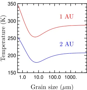
Figure 3. Temperature of a single dust grain as a function of grain size and distance. The temperature decreases with distance as the stellar flux is reduced by 1/r2. The
tempera-ture roughly decreases with grain size, as the grain becomes a better emitter. For grains much larger than the wavelength of emission, the temperature becomes constant as the opacity becomes Grey over the wavelength range where there is sig-nificant absorption and emission.
4.2 Non-equilibrium dust grains
For very small grains in a diluted radiation field, like PAHs in the outer regions of a disk for instance, it is impossible to define a temperature. Small grains have small heat capacities and the absorption of a single UV photon can increase the grain temperature by a substantial amount. These small grains never reach an equilibrium temperature but undergo temperature fluctuations: they heat up very quickly when they absorb a photon and cool down progressively between 2 absorptions. As a consequence they emit on a much broader wavelength range than the one they would emit on if they were at equilibrium. For such transiently heated dust grains, the emissivity (Eq. 21) can be written:
jν=αν
∞
0
P(T)Bν(T) dT (30)
whereP(T) is the probability density of the dust grain to be at a temperature T. Note that in practice, the integral stops at a maximum temperature above which the dust grain is sublimated. This probabil-ity densprobabil-ity depends on the dust grain opacprobabil-ity and heat capacprobabil-ity as well as the hardness and dilution of the radiation field. Several methods exist to compute this probability density (e.g. Desert et al. 1986; Guhathakurta & Draine 1989; Leger & Puget 1984; Siebenmorgen & Kruegel 1992).
4.3 Scattering
Including light scattering strongly increases the complexity of the radiative transfer. Scattering is simultaneously a sink and a source term. Energy is scattered away from the beam, while energy is also scattered into the beam from all the other directions.
The radiative transfer equation becomes an integro-differential equation which relates the radiation fields at all positions and in all different directions:
dIν(s,→−n) ds =−α
ext
ν (s)Iν(s,→−n) +αabs
ν (s)Bν(T(s)) (31)
+αscatt ν (s)
1 4π
Ωψν(s, − →n,→−n)I
ν(s,→−n)dΩ
whereαext = αabsν +ανsca, αabsν andαscaν are the extinction, absorption and scattering cross section respectively. The ratio of the scattering and extinction cross sections is called thealbedo:
ην= α sca ν αabs
ν +αscaν
ψν(s,→−n,→−n) is the scattering phase function, which describes the anisotropy of scattering. It gives the probability that a photon incoming from the direction→−nwill be scattered towards the direction −
→n. This means that we need to solve the radiative transfer equation along all rays at the same time, as we need to knowIν(s,→−n) for all the directions→−nin order to solveIν(s,→−n).
4.4 Radiative transfer of polarised light
The specific intensity only describes unpolarised light. Scattering on dust grains produces polari-sation and aligned dust grains result in polaripolari-sation by emission and dichroïc absorption. Several formalisms exist to describe polarised light, one of the most commonly used uses the Stokes vector S=(I,Q,U,V), whereIis the total specific intensity,QandUdescribe the linearly polarised inten-sity andVthe circularly polarised intensity. The radiative transfer equation can be easily extended in this formalism to account for polarisation:
dSν(s,→−n)
ds =−α
ext
ν (s)Sν(s,→−n) +αabs
ν (s)Bν(T(s)) (33)
+αscatt ν (s)
1 4π
ΩMν(s, − →n,→−n)S
ν(s,→−n)dΩ
The modification from the non-polarised radiative transfer equation are two-fold:
• the absorption and extinction coefficient are becoming vectorial to account for the polarised emis-sion and dicroïc extinction from preferentially aligned grains
• the phase function is replaced by the Mueller matrix (see a full description in Bohren & Huffman 1983; van de Hulst 1981 and Min 2015).
5 Why is radiative transfer difficult ?
In an optically thin medium, for instance a debris disk, solving the radiative transfer and dust temper-ature is easy. The radiation field is dominated at any point by the stellar radiation field, which also sets the dust temperature.
When the medium is optically thick however, like in a protoplanetary disk, optical depths effects strongly increase the complexity of the problem: In some part of the volume, the stellar radiation will be strongly extinct and the specific intensity can be dominant, depending on the position and wavelength, either by the scattering term or the thermal emission term, which both depend on the radiation field at any other points in the volume.
We can summarize this extra complexity by rewriting the previously described equations:
dIν(s) ds =α
ext
ν (s) [Sν(s)−Iν(s)] (34)
and
Sν(s)=Semission
ν (s)+Sνscattering(s) (35)
=αabs
ν (s)Bν(T(s))+αscattν (s) 1 4π
Ωψν(s, − →n,→−n)I
∞
0
Jν(s) dν=
∞
0
Bν(T(s)) dν with Jν(s)= 1 4π
ΩIν(s, −
→n)dΩ (37)
The intensity at any pointIν(s) depends on the source functionSν(s), which in turn depends on the specific intensity in any other direction, and coming from any other point in the model, both for emission and scattering source function. Equations 34 and 35 must be solved simultaneously.
6 Methods to solve the continuum radiative transfer
In this section, we briefly list the various methods that have been used to solve the continuum radia-tive transfer. We focus more on the Monte Carlo method as it seems to be become used more and more widely thanks to its flexibility and the development of new algorithms strongly improving its efficiency.
There are 2 main methods to solve the continuum radiative transfer, which differ in the way they deal with the angular dependence of the radiation field. Discrete ordinate (or ray-tracing) methods use a set of fixed directions on which they solve the radiative transfer equation, and Monte Carlo randomly samples all the directions by following photon packages.
The last decade has seen considerable progress in the development of RT techniques, going from 1+1D models (Chiang & Goldreich 1997), with only vertical transport of radiation and often grey opacities, to more complex models, 2 or 3D with more realistic opacities and treatment of scattered light. Monte Carlo (MC) codes, thanks to their high flexibility, seem to become the rule in the mod-eling of continuum emission, in particular in the field of protoplanetary disks. Only a couple of ray-based have been developed to study disks: RADICAL (Dullemond et al. 2002), ProDiMo (Woitke et al. 2009) HO-CHUNK (Whitney & Hartmann 1992), while there is now a relatively large number of MC-based radiative transfer codes in this field: MC3D (Wolf 2003), TORUS (Harries et al. 2004), MOCASSIN (Ercolano et al. 2005), MCFOST (Pinte et al. 2009, 2006), MCMax (Min et al. 2009).
6.1 Discrete ordinate methods or ray-tracing methods
6.1.1 Lambda iteration
The Lambda iteration is a conceptually simple method to solve the radiative transfer. Basically, it iterates between a global calculation (the radiative transfer equation) and a local calculation (the cal-culation of the source function) until convergence is reached.
The formal solution of the radiative transfer equation 34 can be written via the linearΛoperator:
Jν= Λν[Sν] (38)
As we discussed it before, the formal solution of the RT equation and hence theΛoperator is not a local operation but involves integral over the entire volume. The simple idea between theΛiteration is to iterate between equations 35 and 38: first, a guess on the source function is made, the formal radiative transfer equation is solved on a set of rays, allowing to computeJνfromSν1, finally a new
source function at any point is computed from the local specific intensity, and the whole procedure is iterated.
Each iteration transports the radiation further by about a mean photon free path, meaning that the
To overcome this difficulty, several accelerations can be used, in particular the Accelerated Λ Iteration(ALI, Cannon 1973; Collison & Fix 1991; Hubeny 2003) which splits theΛoperator into an approximateΛ∗operator, which is easy or easier to invert, and the difference between the true and approximateΛoperators:
Λ = Λ∗+(Λ−Λ∗) (39)
A typical choice forΛ∗is the diagonal or tridiagonal ofΛ. This allows to separate the self-coupling of the cells with themselves (diagonal operator) and with their close neighbors (tridiagonal operator), which is now solved by a matrix inversion, from the global calculation. This results in a dramatic speed-up of the convergence of the iteration procedure.
Furthermore, ALI methods can be coupled with additional acceleration such as the Ng-acceleration (Dullemond & Dominik 2004; Ng 1974).
6.1.2 Moment method
In section 2.3, we have introduced the first 3 moments of the specific intensity. If we integrate the radiative equation over all the angles and then multiply by the directional vector and integrate again, we obtain the 2 first moment equations:
dHν
ds = jν(s)−αν(s)Jν(s) (40)
and
dKν
ds =−αν(s)Hν(s) (41)
These equations represent a non-closed system, with more unknowns than equations and we would need an infinite number of equations to end up with a system equivalent to the full angle-dependent radiative transfer equation. In practice, this system is truncated by introducing a closure equation, for instance the Eddington approximation:
Ki,j,ν= 1
3δi,jJν (42)
which is a good approximation for an isotropic radiation field. The equation system can then be reduced to one equation, which is easy to solve numerically with standard numerical methods:
1 3∇
1
αν∇Jν
=αν[Jν−Sν] (43)
This is the diffusion approximation method.
The Variable Eddington Tensor (VET) method (Mihalas & Mihalas 1984) generalizes such an approach, by computing the coefficients fi,j,νin
Ki,j,ν= fi,j,νJν (44)
x
y z
Star random
walk
circumstellar environment
stellar packet
thermal packet emitted by the disc
limit of the model
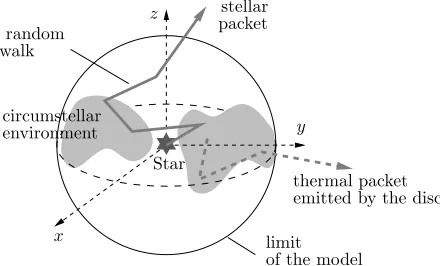
Figure 4.Schematic view of the path of pho-ton packets in a MC code. Packets perform a random walked with absorption and scatter-ing events and eventually escape from the cir-cumstellar medium. Full line represents the path of a stellar packet while the dashed line displays the path of a thermal packet emitted by the disk.
6.2 Monte Carlo method
An alternative method to solve the radiative transfer problem is called the Monte Carlo method. Monte Carlo methods are numerical algorithms which can simulate random processes (Markov chains, trans-port model, finance, . . . ) but also completely deterministic problems, by building a probabilistic model. It is for instance well suited for multi-dimensional integrals. The generally accepted birthdate for this method is 1949 when Metropolis and Ulam published an article “The Monte Carlo” method.
In the case of radiative transfer, the basic idea is to propagate many photon packets by randomly sampling from probability distribution functions for directions, frequencies, path lengths, interactions. Essentially, a Monte Carlo radiative transfer code generates packets and follows them individually, one interaction event after another until they exit the system and reach a detector. All the para-meters of the photon random walk are obtained by drawing random numbers following probability distribution function that reflects the local properties (optical depth, albedo, scattering phase function, temperature, . . . ). This procedure is repeated for a large number of photon packets until the desired convergence is reached.
The Monte Carlo scheme estimates physical quantities by statistical means, which potentially leads to noisy results when the number of packets sampling some regions and/or directions in the model becomes low. Several variance reduction techniques have been developed to improve the sam-pling of the Monte Carlo method: forced first scattering (Cashwell & Everett 1959), peel-off tech-niques (Yusef-Zadeh et al. 1984), estimation of the mean specific intensity (Lucy 1999), immediate re-emission (Bjorkman & Wood 2001), polychromatic packets (Ercolano et al. 2005), importance weighting schemes (Juvela 2005; Pinte et al. 2006), partial diffusion approximation and modified random walk (Min et al. 2009), estimation of the scattering source function and combination with ray-tracing (Min et al. 2009; Pinte et al. 2009). These various techniques allowed the Monte Carlo method to progressively become competitive against grid-based methods, and it is now more and more commonly used to solve the continuum RT problem.
The Monte Carlo has also the strong advantage that it mimics the propagation of photons (Fig. 4), making them intrinsically 3D, and thus making it easier to implement additional physics, whereas the complexity of a discrete ordinate code increases dramatically with dimension.
6.2.1 How to choose random variables from any probability distribution function ?
0 90 180 0.001
0.01 0.1
Scattering angle
θ
S
11(
θ
)
0 90 180
0.2 0.4 0.6 0.8 1.0
Scattering angle
θ
π0
S
11(
θ
) sin(
θ
) d
θ
A
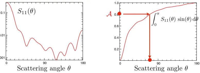
Figure 5.Illustration of the sampling of a probability distribution in a MC code.Left panel: phase function to be sampled. Note that this is the phase of a single grain computed using the Mie theory. This is not a realistic representation of a phase function of dust grains in a disk and is just chosen for illustration here. Right panel: integrated probability distribution function. A random numberAis chosen, the corresponding scattering angle of the valueθfor which0θS11(θ) sinθdθ/
π
0 S11(θ
) sinθdθ=Ais obtained.
the Monte Carlo method. If a set of random variablesAifollows a uniform distribution, the random variablesXi=F−1(A1) follow the distributionf, with
F(x)=
x
a
f(y) dy and
b
a
f(y) dy=1. (45)
One of the main quantities to compute in a Monte Carlo is the distance that a packet will travel up to its next interaction with a dust grain. The fraction of packets that will interact betweenτand
τ+dτis given byP(τ) dτ =e−τ−e−(τ+dτ)dτ. The probability distribution for the optical depthτis
then given by:
P(τ)=e−τ (46)
The optical depth to the next interaction by is then:
τ=−ln(1− A) (47)
The free pathluntil the next interaction is then obtained by integrating:
τ=
l
0
κext(s) ds (48)
This equation is solved by propagating the packet in the medium and adding the opacity along the path until the optical depthτis reached. This is usually the most computing intensive part of a Monte Carlo code and this integration must be performed with care to insure accurate numerical results.
For most probability distributions, an analytic integration, like Eq. 47, is usually not possible and a numerical integration of Eq. 45 is performed instead as illustrated in Fig. 5.
6.2.2 Drawbacks of the basic Monte Carlo method
• First, in the basic Monte Carlo method that we described earlier, one still needs to iterate between JνandT to reach convergence. When a packet interact with dust, it is either scattered or absorbed depending on the local albedo. If it is scattered, its new direction is chosen following the local phase function and it continues its path. But if it is absorbed, the packet is destroyed and its energy2is
stored in the cell. After all the packets of the given iteration have been propagated, the absorbed energy must be re-emitted in the following iteration. When the optical depth becomes large, this procedure suffers the same convergence issue as ALI method and requires an increasingly large number of iterations.
• When the probability of interaction becomes very large, a packet will interact a very large number of times with the medium, for a very small physical propagation through the medium.
• When the probability of interaction becomes small, packets simply go through the medium without interacting,i.e. without producing any information. A large number of packet becomes necessary to properly sample these regions.
• When the observer looks at the disk from a direction where very few packet end up. This is the case for edge-on disk for instance. The probability of packets to scatter in the exact direction becomes very small, requiring again a large number of packets in order to get a statistically correct answer.
Several algorithms have been developed in the last few years to overcome these difficulties, we briefly describe a few important ones in the following section.
6.2.3 Immediate re-emission
One of the major optimization of the Monte Carlo method was introduced by Bjorkman & Wood (2001). The basic idea is to re-emit a packet as soon as it is absorbed. This ensures perfect energy conservation. An absorption/re-emission event is then similar to a scattering event, with the diff er-ence that the re-emission is isotropic and that the packet must change frequency3following the local
emissivity and hence the local temperature.
Choosing the new frequency is actually not easy, as we require that at the end of the simulation, all the packets emerging from a cellimust have been emitted following:
P(ν) dν= jiνdν=αiνBν(Ti) dν (49)
whereTiis the final temperature at the simulation. The problem is of course that we do not knowTi before all the packets have been propagated.
The “trick” invented by Bjorkman & Wood (2001) relies on the fact that a given packet emitted from the celli does not need to be drawn from this probability distribution, as long as the set of all the packets is. Instead, Bjorkman & Wood (2001) use a different probability for each packet. If we assume that a packet is absorbed in a celliwhich so far has absorbed npackets, is at a current temperatureTiand has re-emitted thenprevious packets following jν,n =αiνBν(Ti). When the new packet is absorbed, the temperature increases toTi+δT. Then+1 packets so far absorbed must then be re-emitted followingjν,n+1=ανiBν(Ti+δT).
BecauseBν(Ti+δT)> Bν(Ti) for allν, we also have jν,n+1 > jν,n for allν, and we can consider δjν= jν,n+1−jν,n>0 like a probability distribution. We can then re-emit then+1thpacket following:
δjν= jν,n+1−jν,n=αiν(Bν(Ti+δT)−Bν(Ti))≈αiν
dBν(T)
dT
Ti
(50)
2or more exactly, its luminosity,i.e.energy per second
λ
1 10 100
κλ Bλ
N,T N + 1,
T + ΔT
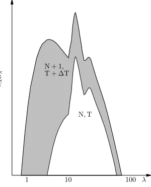
Figure 6. Selection of the wavelength in the imme-diate re-emission algorithm. Emissivity is plotted be-fore (lower curve) and after the absorption of an indi-vidual packet (upper curve). The spectral distribution of the previously distributed packets is represented by the white area. To correct the spectral distribution, the new packet must be emitted following the difference of the 2 curves,i.e.following the shaded area.
The difference can be approximated as a differential asδT will be small if a large enough number of packets is used. This procedure is illustrated in Figure 6. The general mathematical basis for the Bjorkman & Wood (2001) calculation are discussed in details in Baes et al. (2005).
6.2.4 Computing the mean intensity
In the basic Monte Carlo method, the thermal balance in a given cell is performed by equating the energy to re-emit to sum of the energies of all the absorbed packets in the cell.
A much more effective method, introduced by Lucy (1999), is to directly use Eq. 29 by computing the mean intensity from the Monte Carlo run:
Jν= 1
4πViΣγγΔ
lγ (51)
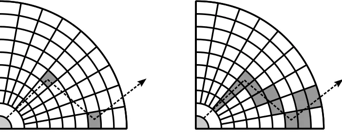
whereγindicates a packet,γ is the packet luminosity andΔlγ is the length the packet propagated through in the celli. Each packet crossing a cell is then contributing to the local mean intensity, as illustrated in Fig. 7. In particular, this allows to very efficiently compute the temperature in optically thin cells where absorption is very unlikely to happen.
6.2.5 Modified random-walk and partial diffusion approximation
In very optically thick regions, solving the radiative transfer via a Monte Carlo method becomes extremely challenging. Photon packets can interact many times (several millions for the optical depths encountered in protoplanetary disks) before exiting the system, increasing the computational times by several orders of magnitude. Min et al. (2009) introduced two complementary methods to speed up the calculations in high optical depth regions: the modified random walk (MRW), simplified by Robitaille (2010), and the partial diffusion approximation (PDA).
Figure 7. Information created by a packet during its propagation. Left: In the basic Monte Carlo method, information is created only in cells where the packet interacts with the medium. Right: using the concept of specific and/or mean intensity allows creating information in all the cells crossed by the packet, resulting in a much lower number of packets required to reach a given convergence, in particular in the optically thin regions of the model.
following a random walk. Using the diffusion approximation, we can then move the packet to the edge of the sphere in a single step. The actual distance propagated by the packet4 can be sampled from a
probability distribution, which depends on the radius of the sphere and on the diffusion coefficient. The photon is then re-emitted from a random position on the sphere, at a wavelength sampled from the source function,i.e.from the Planck function (as we are in a very optically thick region and LTE can be assumed), or from its temperature derivative if the Bjorkman & Wood (2001) method is used. The procedure is repeated until the packet gets close enough to one edge of the cell, and a classical Monte Carlo propagation step can be used.
The PDA can additionally be used after the Monte Carlo run to compute the temperature structure in cells where a small number of packets have travelled. The temperature structure can then be solved using:
∇.(D∇)=0 (52)
whereD = 1/3ρκR is the local diffusion coefficient withκR the local Rosseland opacity, and = 4σT4/cis the energy density, or more simply:
∇.(D∇T4)=0 (53)
This is a system of linear equation which can be solved very quickly, using the Monte Carlo temper-ature as a boundary condition. Note that continuum observations usually do not require this step, as it is used in regions which are not seen by the observer. The main goal of the PDA is to to obtain a reliable temperature structure at any point in the disk, for instance to compute the vertical hydrostatic equilibrium or the chemistry in the disk midplane.
6.2.6 Scattered specific intensity and ray-tracing
The basic Monte Carlo builds images and SEDs by putting detectors in a given direction. The prob-ability of a packet to reach this detector is small. This is compensated by running large (a few 10 to
100 millions) packets to ensure that enough of them will reach the observer. But for a specific con-figuration and wavelength, for instance an optically edge-on disk in the mid-IR, the probability of a packet reaching the observer is so small that it would require prohibitively long CPU-time to compute an emerging flux.
To avoid this, ray-tracing has for instance been used in combination with Monte Carlo methods to produce SEDs and emission maps in the infrared and millimetre regimes, where scattering can be considered isotropic in some cases (Dullemond & Dominik 2004; Wolf 2003). When the scattering is isotropic, only the mean specific intensity and temperature structure are required to calculate the source function. These two quantities can be easily estimated with a Monte Carlo method (Lucy 1999) as discussed before and do not require a large amount of memory to be stored. After an initial Monte Carlo run computing the total mean intensity and temperature structure in the disk, SEDs and/or maps can then be produced by integrating the source function of rays originating from the observer. Which such a method, the Monte Carlo method is only used to estimate the specific intensity, but not the images and/or SEDs. The resulting noise in the observables is much lower as it only reflects the noise in the mean specific intensity.
This method of combining Monte Carlo and ray-tracing can be extended to any wavelength if the angular dependence of the scattering component of the source function is preserved in the calculations (Min et al. 2009; Pinte et al. 2009). The Monte Carlo method produces all the information needed to perform such calculations, as it can give an estimate of the specific intensity, with its complete angular dependence, and not only of the mean specific intensity.
As a packet crosses a cell, we add its contribution to the specific intensity in a given direction for the given cell. Note that we need the full angular dependence of the specific intensity for each cell, i.e. Iν(x, y,z, θ, φ). This requires a large amount of memory and is only possible in practice for models with an azimuthal symmetry. For 3D models, an alternative is to set in advance the directions from where you wish to observe the disk, and store the scattered emissivity instead of the specific intensity. This makes the problem much more tractable but requires to rerun a Monte Carlo calculation for each new direction.
In both cases, at the end of the Monte Carlo calculations,i.e.once the specific intensity or scattered emissivity is known, as well as the dust temperature in any cell of the disk, it is possible to formally integrate the radiative transfer equation along the rays originating from the observer.
7 Conclusion
The continuum radiative transfer represent a complex numerical problem, in particular in protoplane-tary disks where extremely high optical depths can be reached. The Monte Carlo method has become the method of choice to solve this problem in the last few years. With the development of recent al-gorithms, modern radiative transfer codes have become highly flexible, extremely robust numerically, and reasonably fast, allowing the exploration of a significant fraction of the parameter space when comparing model with observations.
AcknowledgementsThe research leading to these results has received funding from the European Union Seventh Framework Programme FP7-2011 under grant agreement no 284405.
References
Baes, M., Stamatellos, D., Davies, J. I., et al. 2005, New Astronomy, 10, 523
Degree of linear polarization
Monte-Carlo 30s
MC + ray-tracing 3s
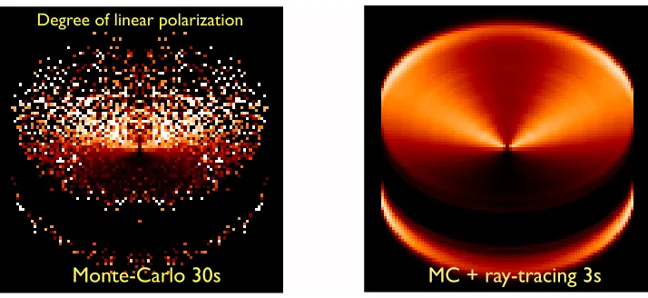
Figure 8.Comparison of polarization maps obtained using the classical photon collecting method (left) and the Monte Carlo+ray-tracing method (right).
Bohren, C. F. & Huffman, D. R. 1983, Absorption and scattering of light by small particles (New York: Wiley, 1983)
Cannon, C. J. 1973, J. Quant. Spec. Radiat. Transf., 13, 1011
Cashwell, E. & Everett, C. 1959, A practical manual on the Monte Carlo Method for random walk problem (Pergamon Press, New York)
Chiang, E. I. & Goldreich, P. 1997, ApJ, 490, 368
Collison, A. J. & Fix, J. D. 1991, BAAS, 23, 1410
Desert, F. X., Boulanger, F., & Shore, S. N. 1986, A&A, 160, 295
Dullemond, C. P. & Dominik, C. 2004, A&A, 421, 1075
Dullemond, C. P., van Zadelhoff, G. J., & Natta, A. 2002, A&A, 389, 464
Ercolano, B., Barlow, M. J., & Storey, P. J. 2005, MNRAS, 362, 1038
Guhathakurta, P. & Draine, B. T. 1989, ApJ, 345, 230
Harries, T. J. 2011, MNRAS, 416, 1500
Harries, T. J., Monnier, J. D., Symington, N. H., & Kurosawa, R. 2004, MNRAS, 350, 565
Hubeny, I. 2003, in Astronomical Society of the Pacific Conference Series, Vol. 288, Stellar Atmo-sphere Modeling, ed. I. Hubeny, D. Mihalas, & K. Werner, 17
Juvela, M. 2005, A&A, 440, 531
Leger, A. & Puget, J. L. 1984, A&A, 137, L5
Lucy, L. B. 1999, A&A, 344, 282
Mihalas, D. & Mihalas, B. W. 1984, ApJ, 283, 469
Min, M. 2015, in EPJ Web of Conferences, Vol. 102, Summer School on Protoplanetary Disks: Theory and Modeling Meet Observations, ed. I. Kamp, P. Woitke, & J. D. Ilee
Min, M., Dullemond, C. P., Dominik, C., de Koter, A., & Hovenier, J. W. 2009, ArXiv e-prints
Ng, K.-C. 1974, J. Chem. Phys., 61, 2680
Pinte, C., Harries, T. J., Min, M., et al. 2009, A&A, 498, 967
Pinte, C., Ménard, F., Duchêne, G., & Bastien, P. 2006, A&A, 459, 797
Robitaille, T. P. 2010, A&A, 520, A70
Siebenmorgen, R. & Kruegel, E. 1992, A&A, 259, 614
van de Hulst, H. C. 1981, Light scattering by small particles (New York: Dover, 1981)
Whitney, B. A. & Hartmann, L. 1992, ApJ, 395, 529
Woitke, P., Kamp, I., & Thi, W. 2009, A&A, 501, 383
Wolf, S. 2003, Computer Physics Communications, 150, 99