Maklaya str. 6, Moscow, 117198, Russia
Abstract.A local variation in the thickness of the waveguide layer of integrated optics waveguide causes a local decrease of phase velocity, and hence bending of rays and of the wave front. The relationship of the waveguide layer thickness profileh(y,z) with the distribution of the effective refractive index of the waveguideβ(y,z) is described in terms of a particular model of waveguide solutions of the Maxwell equations. In the model of comparison waveguides the support of the thickness irregularity of the waveguide layer
Δhcoincides with the support of inhomogeneity of the effective refractive indexΔβ. A more adequate but more cumbersome model of the adiabatic waveguide modes allows them to mismatch suppΔh ⊃ suppΔβ. In this paper, we solve the problem of theΔh reconstruction on the base of givenΔβof the thin film generalized waveguide Luneburg lens in a model of adiabatic waveguide modes. The solution is found in the form of a linear combination of Gaussian exponential functions and in the form of a cubic spline for the cylindrically symmetricΔh(r) and in the form of a cubic spline forΔβ(r).
1 Introduction
The method of adiabatic waveguide modes proposed in [1, 2] reduces the boundary problem for a sys-tem of partial differential equations to the problem for a system of ordinary differential equations. The adiabatic waveguide modes of a smoothly irregular waveguide satisfy the exact boundary conditions on the inclined planes, tangent to the interface between two media, so that the system of ordinary differential equations for vertical distributions of the electromagnetic fields of the modes takes the form of two coupled oscillators for two polarizations of the electromagnetic field of the TE and TM modes. As an example, consider a dielectric waveguide of the following structure (figure 1).
In the regular part of the waveguide, a waveguide guided TE (TM) mode of the form ⎛
⎜⎜⎜⎜⎜ ⎜⎜⎜⎜⎝ E
j y Hxj Hzj
⎞ ⎟⎟⎟⎟⎟
⎟⎟⎟⎟⎠(x) expiωt−iβjk0z ,
⎛ ⎜⎜⎜⎜⎜ ⎜⎜⎜⎜⎝ E
j x Ezj Hyj
⎞ ⎟⎟⎟⎟⎟
⎟⎟⎟⎟⎠(x) expiωt−iβjk0z ae-mail: ayrjan@jinr.ru
be-mail: genin_d@mail.ru ce-mail: lovetskiy@gmail.com de-mail: alsevastyanov@gmail.com
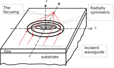
Figure 1.Schematic representation of (thin-film generalized waveguide lens) Luneburg TGWL
propagates along the axisOzto infinity. In the vicinity of the origin, the waveguide mode runs across an irregularity of the waveguide formed by an additional waveguide layer with variable thickness h(r) and cylindrically symmetric with respect to the axisOx. The phase velocity of the wave front (lines of constant phase) slows down (larger deceleration takes place closer to the origin, smaller – at increasing distances from the origin), and two-dimensional “rays”, locally orthogonal to the fronts, acquire local curvature toward the axisOz. If the profileh(r) is selected properly, all the rays that have passed through the region of irregularity of the waveguide gather in the focal point on the axisOzat a distanceFfrom the origin. Turning the incident beam of rays (the direction of the incoming regular waveguide mode) around the axisOx, we get an identical pattern: the focal point moves by the same angle along a “big” circle of radiusF. Thus, the described irregularity of the waveguide forms the structure of a “Luneburg waveguide lens” that is, a two-dimensional Luneburg lens for the original waveguide mode of the regular waveguide.
2 Luneburg lens
The Luneburg lens was proposed by RK Luneburg in his course on the Maxwell optics [3]. It is described in terms of geometrical optics in a three-dimensional (or two-dimensional) space filled by a medium (or vacuum) with given permittivity and permeability, such that the optical density is uniform. In the vicinity of the origin inside the sphere (disk) of radiusRthe optical densityn(r) (and thereforeε(r),μ(r)) is not uniform, increasing toward the origin so that the parallel light beam after passing through the region of «n» inhomogeneity focuses on the distanceF ≥Rfrom the origin of coordinates. IfF=Rthe Luneburg lens is called classical, it is realized provided
n(r)=nc2−(r/R)2.
IfF>Rthe Luneburg lens is called generalized andn(r) satisfies the integral relations [4]:
n(r)=exp [ω(ρ,F)], where ρ=rn(r) and ω(ρ,F)= 1
π
π
ρ
arcsin(x/F) (x2−ρ2)(1/2)dx.
The angular aperture of the a classical Luneburg lens isΩ =180◦ =π. In the generalized Luneburg lens the angular aperture equalsΩ =2arctg (R/F) and depends on the focal distance [7]. The shorter the focus, the larger the aperture, and lim
are described by special case mappings
(E,H)T : R3×R→R6,
(x, y,z,t)T→ Ex,Ey,Ez,Hx,Hy,HzT(x, y,z,t)T.
Assuming an electromagnetic field of a fixed frequencyω, we introduce the dimensionless “normal-ized” coordinates by setting the normalization (x, y,z,t)T → x˜,y,˜ z˜,t˜T, where ˜
x = k0x, ˜y = k0y,
˜
z= k0z, ˜t =ωt, withk0 =ω/c,cis the speed of light in vacuum, so that ˜k0 = 1, ˜ω =1, ˜c=1 in
new “normalized” coordinates (variables). The field intensities will then be measured in fractions of “amplitude” intensity of the incoming light flux
Ej,Hk
→ Ej √
I,Hk√I≡E˜j,Hk˜ .
In terms of the normalized variables, the Maxwell equations take the form:
rot˜H=iε˜˜E, rot˜E=−iμ˜˜H, (1)
where
˜H≡ ˜Hωx˜,y,˜ z˜,t˜, ˜E≡ ˜Eωx˜,y,˜ ˜z,t˜, ˜
ε≡ε˜ω( ˜x,y,˜ z˜)≡εω(x, y,z), μ˜ ≡μ˜ω( ˜x,y,˜ z˜)≡μω(x, y,z). Tangential boundary conditions at the interface between two media can be written as:
˜Hτ
1= ˜H
τ
2, ˜E
τ
1 = ˜E
τ
2. (2)
At infinitely remote distance the asymptotic conditions for the tangential components of the electro-magnetic field are:
˜Eτ
x→±∞<+∞, ˜Hτx→±∞<+∞. The solutions of (1) for adiabatic waveguide modes are sought in the form:
˜E ˜ x,y,˜ z˜,t˜
˜Hx˜,y,˜ z˜,t˜
=
˜E ( ˜x; ˜y,z˜)
˜H( ˜x; ˜y,˜z)
expit˜−iϕ˜(˜y,z˜)
˜
β(˜y,z˜) , where
˜
βy(˜y,z˜)=
∂ϕ˜
∂y˜
, β˜z(˜y,z˜)=
∂ϕ˜
∂z˜
, and β˜(˜y,z˜)=
˜
βy(˜y,z˜)2+β˜z(˜y,z˜)2.
4 Waveguide fields and boundary conditions in the zero approximation
In the multilayer waveguide, in the zero approximation, the equations for the longitudinal components of the electromagnetic field of the adiabatic waveguide modes take the form [5–7]:
d2E˜0
z dx˜2 +
˜
εμ˜−β˜2E˜0
z =0, (3)
d2H˜0
z dx˜2 +
˜
εμ˜−β˜2H˜z0=0. (4)
The expressions for the other four components of the electromagnetic field take the form:
˜ H0
x= (ε˜μ−˜1β˜2
z)
−iβ˜zd
˜
H0
z
dx˜ +ε˜β˜yE˜0z
, H˜0
y= (ε˜μ−˜1β˜2
z)
−iε˜dE˜0z
dx˜ −β˜zβ˜yH˜z0
,
˜ E0
x=(ε˜μ−˜1β˜2
z)
−iβ˜zdE˜0z
dx˜ −μ˜β˜yH˜z0
, E˜0
y= (ε˜μ−˜1β˜2
z)
i˜μdH˜0z
dx˜ −β˜zβ˜yE˜z0
. (5)
In the subdomains (waveguide layers) with constant refractive indicesn2
j =εjμjthe solutions ˜E0z of the fundamental system (3) are written as:
˜
Ezs=As˜ exp{γ˜s( ˜x−a˜1)}, E˜zf =A˜+fexp
iχ˜f( ˜x−a˜2) +A˜−f exp
−iχ˜f( ˜x−a˜2) ,
˜ El
z=A˜+l exp
iχ˜l
˜
x−a˜2−h˜ +A˜−l exp
−iχ˜l
˜
x−a˜2−h˜ , E˜cz =Ac˜ exp
−γ˜c
˜
x−a˜2−h˜ .
(6)
while the solutions ˜H0
z of (4) in the form:
˜ Hs
z =Bs˜ exp{γ˜s( ˜x−a˜1)}, H˜zf =B˜+f exp
iχ˜f( ˜x−a˜2) +B˜−fexp
−iχ˜f( ˜x−a˜2) ,
˜ Hl
z=B˜+l exp
iχ˜lx˜−a˜2−h˜ +B˜−l exp
−iχ˜lx˜−a˜2−h˜ , H˜zc=Bc˜ exp
−γ˜cx˜−a˜2−h˜ .
(7)
Substituting (6)–(7) into (5), we obtain expressions for the other four components of the electromag-netic field. The substitution of all of them in the boundary equations (2) will result in expressions which, after reducing similar terms, give a system of homogeneous linear algebraic equations for the undefined amplitude coefficients ˜As,Bs˜ ,A˜±f,B˜±f,A˜±l,B˜±l,Ac˜ ,Bc˜ . This system which is characterized by a matrixM(β), can have non-trivial solutions provided [6, 8]
detM(β(r))=0. (8)
5 A thin-film generalized waveguide Luneburg lens synthesis
The solution of a given nonlinear PDE of the first order with respect toh(r) resolves the proper profile of the Luneburg TGWL.
Southwell [9] has solved the thickness profile of a Luneburg TGWL with parametersns =1.47, nf =1.565,nl=2.10,nc=1.0,d =1.0665μ,λ=0.5μby the method of comparison waveguides in which the precise boundary conditions for the Maxwell equations are replaced by their approximations – projections on the horizontal plane [10]. We repeated these calculations for the focal lengths given in [9]. The support of the irregularity region of TGWL in the method of comparison waveguides automatically coincides with the support ofnejff(r)=βj(r)/βjinhomogeneity of the two-dimensional TGWL of Luneburg: supph=suppn=suppβ.
ds ds ∂y ds ds ∂z
using the substitutionsdydz =V,A= 1
β∂β∂z,B= 1β∂β∂y, we obtain the equivalent system of ODEs dy
dz =V,
dV dz =
1+V2(B−AV). (9)
The Cauchy problem for the system (8) with the initial conditions
y(z0)=y0, V(z0)=0, (10)
is solved by the Runge-Kutta-Fehlberg method of the 6th order with automatic step selection resulting in the family of “data” yF
j
zkj, VF j
zkj at the family of points automatically generated during the derivation of the solution of the problem (9)-(10) for any beforehand defined focal distance F. Data from the filesyFjzkj,VF
j
zkjallows the calculation of the components of the vector field of the phase
delayβ=βz, βy T
of the AWM for whichβ(y,z)=
β2
y+β2z from
βy
zkj=βzkjVzkj1+V2zkj1/2, βz
zkj=βzkj1+V2zkj1/2. (11)
The result (11) allows to complement the previously generated data file toyFj zkj,VF j
zkj,βFy zkj,
βF z
zkj. Now we have at our disposal all the necessary data for the formulation of the problem of synthesishF(r). The matrix depends on the following variables
MβF=Mns,nf,nl,nc,d, {zkj, ykj,Vkj}, βF
yj k,z
j k
, γF s
yj k,z
j k
, γF c
yj k,z
j k
, χF f
yj k,z
j k
, χF l
yj k,z
j k , βF y yj k,z
j k
, βF z
yj k,z
j k
, hFzj k, y
j k
,∂∂yhF zkj, ykj,∂h F
∂z
zkj, ykj,F.
For the matrixM*,zkj, ykj, . . . ,Fat each point of the “phase-ray mesh{zkj, ykj}F” the condition
detM*,zkj, ykj, . . . ,F=0
has to be fulfilled. The approximationhNF(r) of the functionhF(r) which defines the thickness profile of the irregular waveguide layer, is sought in the form:
hFN(z, y)= N
i=1
Kiexp⎧⎪⎨⎪⎩−(y−yc)
2+(z−zc)2
C2
i
⎫⎪⎬
which allows the explicit calculation of the derivatives. The search for the unknown coefficients (Ki,Ci) to construct an approximate solutionhF(r) in (12) is carried out by minimizing the objective function
Farg(Ki,Ci)=
zkj,yj k detM
⎛
⎜⎜⎜⎜⎝hFN(z, y),∂h F N(z, y)
∂y ,
∂hF N(z, y)
∂z ⎞ ⎟⎟⎟⎟⎠2
by the Nelder-Mead method [8].
6 Conclusion
The paper describes the classical and generalized Luneburg lens in bulk and waveguide implementa-tion. The link between the focusing inhomogeneity of the effective refractive index of the waveguide Luneburg lens and the irregularity of the waveguide layer thickness generating this inhomogeneity is demonstrated. For the dispersion relation of the irregular thin-film waveguide in the AWM model the problem of the “mathematical” synthesis and computer-aided design of the waveguide layer thickness profile for Luneburg TGWL with a given focal length is solved.
The calculations are carried out in normalized (in a special way) coordinates in order to adapt the used relations to computer calculations.
The obtained solution is compared with the same solution within the model of comparison waveg-uides, which is rougher as compared to the AWM model due to the replacement of the exact boundary conditions (for the tangential components of the electromagnetic field) by their projections onto the horizontal plane.
Acknowledgements
The work is partially supported by RFBR grants No’s 13-01-00595 and 14-01-00628.
References
[1] L.A. Sevastianov and A.A. Egorov, Opt. Spectrosc.105, 576 (2008)
[2] A.A. Egorov and L.A. Sevast’yanov, Quantum Electronics39 (6)566–574 (2009) [3] R.K. Luneberg,Mathematical theory of Optics(University of California Press, 1966) [4] S.P. Morgan, J. Appl. Phys.29, 9, 1358–1368 (1958)
[5] E.A. Ayryan, A.A. Egorov, L.A. Sevastianov, K.P. Lovetskiy, and A.L. Sevastyanov, Lecture Notes in Computer Science7125, 136–147 (2012)
[6] A.L. Sevastyanov, Lett. PEPAN8, 804–811 (2011)
[7] A.A. Egorov, L.A. Sevastianov and A.L. Sevastyanov, Quantum Electronics44 (2), 167 (2014) [8] A.A. Egorov, A.L. Sevastyanov, E.A. Ayryan, and L.A. Sevastianov, Matem. Model. 26, 11,
37–44 (2014)
[9] Southwell W.H.JOSA67, 8, 1010–1014 (1977)