Turbulent flow computation in a circular U-Bend

(1)

a

Corresponding author: mohammed.aounallah@univ-usto.dz

Turbulent flow computation in a circular U-Bend

Abdelkrim Miloud1, Mohammed Aounallah1,a, Mustapha Belkadi1, Lahouari Adjlout1, Omar Imine2 and Bachir Imine2

1

Laboratory of Naval Aero-Hydrodynamics, Marine Engineering Department, Faculty of Mechanics, USTO

MB, P.O. 1505 EL-Mnaouar, Algeria.

2

Laboratory of Aeronautics and Propulsive Systems, Mechanical Engineering Department, Faculty of

Mechanics, USTO MB, P.O. 1505 EL-Mnaouar, Algeria.

Abstract. Turbulent flows through a circular 180° curved bend with a curvature ratio of 3.375, defined as the

the bend mean radius to pipe diameter is investigated numerically for a Reynolds number of 4.45×104. The

computation is performed for a U-Bend with full long pipes at the entrance and at the exit. The commercial

ANSYS FLUENT is used to solve the steady Reynolds–Averaged Navier–Stokes (RANS) equations. The

performances of standard k-ε and the second moment closure RSM models are evaluated by comparing their

numerical results against experimental data and testing their capabilities to capture the formation and extend this turbulence driven vortex. It is found that the secondary flows occur in the cross-stream half-plane of such configurations and primarily induced by high anisotropy of the cross-stream turbulent normal stresses near the outer bend.

1 Introduction

Over the last ten years, several numerical studies of fully developed curved-pipe flows are carried out to elucidate the problem of secondary flow patterns in such flows. On the other hand, a substantial amount of experimental information has been obtained for developing turbulent flows in curved ducts [1]. As is known in the literature, the secondary motions in the cross-stream half-plane of developing curved-pipe flows are influenced by different parameters. Among the more important are the curvature ratio, defined as the pipe radius over bend radius of curvature, Reynolds number, defined with respect to pipe diameter and centerline velocity, inlet flow distributions and above all by the condition of the entrance flow, ie; laminar or turbulent [2]. Azzola et al. [3] investigated turbulent curved-pipe flows with different curvature ratio and Re and fully developed turbulent flow at the inlet. The total and circumferential velocity measurements indicated the presence of a center cell near the pipe center witch is confirmed further by the k-ε model calculations of Azzola et al. [4] and Anwer et al [5]. In both these calculations, radial velocity component reversal along the horizontal diameter near the pipe center is found. However, secondary flow separation near the inner bend is not observed. This is a consequence of the secondary boundary layer being turbulent and, therefore, can overcome a larger pressure gradient before separation. As a result, only two secondary cells are found in the

cross-stream half-plane of turbulent curved-pie flows. It is known that Reynolds-stress can generate vorticity in a turbulent flow. The vertical motion thus generated is classified as Prandtl’s secondary flow of the second kind and is referred to as turbulence-driven or stress-induced secondary flow by Bradshaw [6]. This interesting phenomenon is a unique feature of turbulent flow.

From the literature survey, it is found experimentally difficult and expensive to investigate secondary motions in curved-pipe flows, and alternative is to study them numerically. It should be borne in mind that, even in numerical computation, resolution of secondary cells is affected by many factors. Among the more important ones are numerical technique, grid size, and turbulence models. In order to gain an impression of how successful or otherwise the widely used k-ε eddy viscosity model and the RSM are in predicting this flow behavior, the solving scheme developed has provided the basis for a numerical simulation. The objectives of this study are to investigate the effect of the turbulence models: the k-ε and the RSM models. Their performances are evaluated by comparing their numerical results against experimental data and testing their capabilities to capture the formation and extend this turbulence driven vortex.

This is an Open Access article distributed under the terms of the Creative Commons Attribution License 2.0, which permits unrestricted use, distribution, and

C

(2)

2 Problem position

The basic components of the flow test section are shown schematically in Fig. 1. The configuration tested is composed with two straight pipes and a 180 deg. curved pipe. The pipe cross-section was circular throughout with a 4.45 cm inner diameter (D). The ratio of bend mean radius of curvature to pipe diameter was Rc/D = 3.375. Both tangents were of length X = 54.7 D, being, respectively, attached to the 0 deg. (inlet) and 180 deg. (outlet) planes of the bend by means of flanges.

Figure 1. U-Bend geometry features

3 Governing equations

The viscous incompressible turbulent flow is described by Navier-Stokes equations completed by one of the two turbulence models: the standard k-ε and the Reynolds stress model RSM. The mean flow pressure is P and the mean velocity ui.

0 j j x U (1)

j j t j i j j i t j i i j j x u x x u x u x x P u u x 3

2 (2)

3.1. Standard K-ε model

k j k t j j

j x G

k x

u k

x (3)

k C G k C x x u x k j t j j j 2 2 1

(4) 2 k C

t

(5)

Gk represents the production of turbulence kinetic energy

due to the mean velocitygradients and the constantsare: C1ε = 1.44, C2ε = 1.92, Cμ = 0.09, σk = 1.0, σε = 1.3

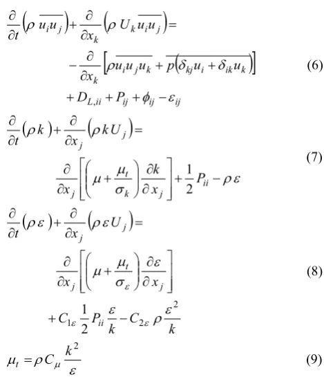
3.2. Reynolds Stress Model RSM

ij ij ij ii L k ik i kj k j i k j i k k j i P D u u p u u u x u u U x u u t ,

(6)

ii j k t j j j P x k x U k x k t 2

1

(7)

k C k P C x x U x t ii j t j j j 2 2 1 2 1 (8) 2 k C

t (9)

DL,ij , Pij do not require any modeling, its represent the

molecular diffusion and the stress production respectively. However, _ijand εij represent the pressure

strain and the dissipation and need to be modeled to close the equations. The constants are: C1ε = 1.0, C2ε = 1.92, Cμ = 0.09, σk = 0.82, σε = 1.0

4 Grid generation

(3)

Figure 2. The hexahedral grid of the U-Bend

5 Numerical approach

The problem treated is a steady three-dimensional turbulent flow through a circular 180° curved bend with a curvature ratio of 3.375. The Reynolds number based on the velocity at the centreline and the diameter of the pipe is fixed to 4.45×104. All the simulations are done with the commercial code: ANSYS Fluent 6.3.26. The segregated implicit solver based on the pressure is used to solve the governing equations of motion. The algorithm Simple is used for coupling pressure-velocity. The full simulations were conducted the 2nd order upwind. The solution converges when the residuals fall down 10-10 for continuity, momentum and turbulence quantities.

.

6 Results and discussion

Figure 3 shows the position of the section where the contours and the profiles of velocity are plotted. The section 1, 2 and 8 are set in the straight pipes following the z axis while sections 3, 4, 5, 6 and 7 are located in the curved part with the appropriate angles showed in the figure.

Figure 3.Location of the reference section

Figure 4shows the wall y+ distribution on the curved part of the U-Bend obtained by both turbulence models. The range of the y+ is obviously adequate with using a high Reynolds number turbulence model. This figure illustrates that the resolution of the grid used is satisfactory with the turbulence model type. Commonly, the two turbulence models predict a largest y+ in the inside region and smallest y+ in the outside of the U-Bend. A clear quantitative difference exists between the predictions of the two models tested mainly in the curved part. This difference is certainly due to difference in the velocity field predicted.

a) k––– model

b) RSM model

(4)

Figure 5 shows the normalized flow velocity (stream wise direction) at different sections obtained with both turbulence models, the velocity is normalized by the reference velocity taken in definition of the Reynolds number, 4.45×104. Scans are made at X/D = 0and 1 in the straight pipes and θ = 3, 45, 90, 135, and 177deg in the bend. The contours are shown as the left part indicates the inside of the tube and the right part designates the outside one. The computed longitudinal velocity component at the section 2, X/D = 1 is identical between both simulations. The forms of the contours are accurately circular and show good agreement with the developed in a straight pipe. At this position, the flow is fully developed in the central region. Close to the wall, the longitudinal velocity tends to zero in respect with the adherence condition.

In the first half of the bend (θ = 3 to 90 deg) as is shown in the section 4, the streamwise velocity contour show a strong deformation of circular forms obtained previously but the features is still symmetric following the horizontal radial axis. The bulk velocity contours tend to be longer in the vertical direction and less large in the horizontal direction. Close to the inside region of the curved pipe, the flow tend to accelerate and contrary to the previous section, notable qualitative discrepancies exist between both predictions obtained by the turbulence models.

The occurrence of a second cross-stream flow reversal past θ = 90 deg in the bend shows a large part dominated by an accelerated flow except the region close to the inside of the curved pipe. From the whole of the contours presented, it is clear seen that location characterizes the maximum reached, that why the surface of the bulk velocity decreases in the coming positions. At θ = 135 deg, the figure shows the core of the streamwise flow neighboring the inside part losing speed while the flow near the inside wall accelerates. According the last section X/D = 1 in the outlet branch of the U-Bend, the flow seem to be accelerated in the half vertical section close to the outside part of the curved pipe. On the other half, the streamwise velocity flow decreases especially near the inside region.

To get more quantitative agreement of the computation, the numerical profiles of the streamwise obtained by both models are compared with the experimental data of Azzola et al. [3] for the different locations cited. A good quantitative agreement is obtained by both turbulence model simulations for the first sections, X/D = 1 and until θ = 3, no great curvature of the U-bend. The numerical results shows a slight over estimation for θ = 45 deg where the increase of the circumferential component of mean velocity at corresponding station reveal the development of a strong secondary flow. At the middle section of the U-Bend, θ = 90, both turbulence models underestimates the stream wise velocity in the first half and over predicts on the second half. At θ = 135, the numerical results seem to be more close to the experimental data, a slight difference

Section 2

Section 4

Section 5

Section 6

Section 8

k~ e model RSM model

(5)

0,0 0,1 0,2 0,3 0,4 0,5 0,0

0,5 1,0 1,5 2,0

Section 1 (X=0)

Normalized flow velocity

R/D

Exp. [3] K-epsilon RSM

0,0 0,1 0,2 0,3 0,4 0,5

0,0 0,5 1,0 1,5 2,0

Section 3 (3 degres)

R/D

Exp.[3] K-epsilon RSM

0,0 0,1 0,2 0,3 0,4 0,5

0,0 0,5 1,0 1,5 2,0

R/D

Exp. [3] K-e model RSM model

Figure 6. Normalized flow velocity for different sections

appear at the central part, while a major discrepancy is shown at the last section X/D =1 in the out coming branch.

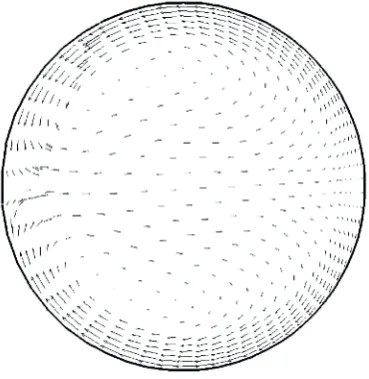
Figure 7 shows the secondary flow vectors in the cross-sectional plane. The increase of the circumferential component of mean velocity at corresponding station reveals the development of a strong secondary flow. The secondary flow is induced by the transverse pressure gradient set up between the outer and inner wall regions of the bend. In the pipe center, it works to overcome and

0,0 0,1 0,2 0,3 0,4 0,5

0,0 0,5 1,0 1,5 2,0

R/D

Exp. [3] k-e model RSM model

0,0 0,1 0,2 0,3 0,4 0,5

0,0 0,5 1,0 1,5 2,0

section 6 (135 degres)

R/D

0,0 0,1 0,2 0,3 0,4 0,5

0,0 0,5 1,0 1,5 2,0

section 8 (x=D)

R/D

(6)

Figure 7. Cross-stream vector at the section θ = 90 deg.

Conclusion

In order to investigate the performance of the turbulence models: the widely used k-ε eddy viscosity and the second order closure RSM to predict reasonably the flow behavior in a 180 deg U-Bend curved pipe at a pipe Reynolds number of 4.45× 104 and a radius ratio of and a radius ratio of 3.375 has been carried. The numerical study reveals that the secondary flow pattern in a curved pipe is very complicated. The results support the notion of an additional (symmetrical) pair of counter-rotating vortical structures embedded in the core of the flow within the curved pipe.

The numerical simulations have reproduced with a gratifying degree of fidelity the measured evolution of the flow with some slight quantitative discrepancies in the curved part of the U-Bend. No significant differences are detected between the two turbulence models tested.

References

1. J. A. C Humphrey, J. H Whitelaw and G. Yee, J. Fluid Mech.,Vol. 103, 443-463 (1981).

2. Y.G. Lai, R.M.C. So and H.S. Zhang, Theoret. Comput. Fluid Dynamics, Vol. 3, 163-180 (1981) 3. J. Azzola and J. A. C Humphrey, Developing

Turbulent Flow in a 180° Curved Pipe and its Downstream Tangent, Report LBL-17681, Materials and Molecular Research Division, Lawrence Berkeley Laboratory, University of California (1984).

4. J. Azzola, J. A. C Humphrey, H. Iacovidas and B.E. Launder, J. Fluids Engrg. 108, 214-221 (1986). 5. M. Anwer, R.M.C. So and Y.G. Lai, Phys. Fluids A

1, 1387-1397 (1989).