Flexible Methods and Computation for Model Selection and Optimal Treatment Learning.

(1)

ABSTRACT

XIAO, WEI. Flexible Methods and Computation for Model Selection and Optimal Treatment Learning. (Under the direction of Wenbin Lu and Hao H. Zhang.)

This dissertation studies the methods and computational algorithm for model selection,

and develops robust estimation method for optimal individualized treatment rules. It contains

four parts. Chapter 1 gives an overall introduction of the thesis. In Chapter 2, we develop a

penalization approach to conduct structure selection for time-varying coefficient Cox models.

Specifically, we propose a method which can simultaneously identify the structure of covariate

effects in a time-varying coefficient Cox model, i.e., covariates with null effect, constant effect and

truly time-varying effect, and estimate the corresponding regression coefficients. Our method

is able to identify the underlying true model structure with probability tending to one and

estimate the time-varying coefficients consistently. The asymptotic normalities of the resulting

estimators for both the constant coefficients and truly time-varying coefficient functions are

also established. We demonstrate the performance of our method using simulations and an

application to the primary biliary cirrhosis data.

In Chapter 3, we further study and develop the computational algorithm for model/variable

selection. We show that the least angle regression (LAR) originally proposed by Efron, Hastie,

Johnstone and Tibshirani (2004) for continuous model selection in linear regression can be

extended in a fruitful way. In particular, we propose a ConvexLAR algorithm that works for

any convex loss function and naturally extends to group selection and data adaptive variable

selection. After simple modification it also yields new exact path algorithms for certain penalty

methods such as a convex loss function with lasso or group lasso penalty. Variable selection

in recurrent event and panel count data analysis, Ada-Boost, and Gaussian graphical model is

reconsidered from the ConvexLAR angle.

In Chapter 4, we develop and study new methodologies to personalized medicine. Because

(2)

increas-ing interest in developincreas-ing individualized treatment. In particular, people are eager to find the

optimal individualized treatment rule, which is a decision rule that if followed by the whole

pa-tient population would lead to the “best” outcome. In this chapter, we propose new estimators

based on robust regression with general loss functions to estimate the optimal individualized

treatment rules. The new estimators possess the following nice properties: first, they are robust

against skewed, heterogeneous, heavy-tailed errors or outliers; second, they are robust against

misspecification of the baseline function; third, under certain situations, the new estimator

cou-pled with pinball loss approximately maximizes the outcomes conditional quantile instead of

conditional mean, which leads to a different optimal individualized treatment rule from the

tra-ditional Q- and A-learning. Consistency and asymptotic normality of the proposed estimators

are established. Their empirical performance is demonstrated via extensive simulation studies

(3)

(4)

Flexible Methods and Computation for Model Selection and Optimal Treatment Learning

by Wei Xiao

A dissertation submitted to the Graduate Faculty of North Carolina State University

in partial fulfillment of the requirements for the Degree of

Doctor of Philosophy

Statistics

Raleigh, North Carolina

2014

APPROVED BY:

Leonard A. Stefanski Arnab Maity

(5)

DEDICATION

(6)

BIOGRAPHY

Wei Xiao was born in Chengdu, Sichuan, China in April 1986. He graduated from Shude High

school in 2004 and attended Fudan University afterwards. He received a Bachelor degree in

statistics in 2008 from Fudan University. In 2009, he was granted a full scholarship in North

Carolina State University to pursue a PhD in statistics. His doctoral dissertation research at

North Carolina State University is under the direction of Dr. Wenbin Lu and Dr. Hao Helen

Zhang. His dissertation focuses on developing flexible methods and computation for model

(7)

ACKNOWLEDGEMENTS

I would like to express my deepest gratitude to my advisors Dr. Wenbin Lu and Dr. Hao

H. Zhang for their enormous support though my graduate study. Their patience, inspiration,

encouragement, enthusiasm, and immense knowledge help me in every step of my dissertation

research. From them, I learned not only statistical knowledge but also the way to conduct a

research. I could not have finished this work without their guidance.

I would also like to extend my appreciation to my committee members, Dr. Leonard A.

Stefanski and Dr. Arnab Maity for their advices, and for the wonderful courses they have

taught me. I owe special thanks to Dr. Yichao Wu and Dr. Hua Zhou. Specifically, Chapter 3

is based on a joint work with them. Their insight and knowledge are invaluable to me, which

bring me to the world of computational statistics. I want also thank Dr. Seth Sullivant, who

agrees to serve as my graduate school representative in both my Ph.D. oral preliminary and

defense out of his busy schedule.

Thanks to Dr. Lexin Li, Dr. Jason A. Osborne, Dr. Daowen Zhang, Dr. David A. Dickey,

Dr. John F. Monahan, Dr. Brian J. Reich, Dr. Min Kang, Dr. Subhashis Ghosal, Dr. Sujit K.

Ghosh, Dr. Anastasios Tsiatis, Dr. Eric Laber, Dr. Ana-Maria Staicu and Dr. Dennis Boos

for teaching me so many useful courses and giving me advices in my research. Thanks to

all my friends at NCSU. The joy we have throughout various parties, sports and travels are

unforgettable.

I would also like to thank Quintiles and SAS Institute Inc. for offering me Graduate

In-dustrial Traineeship (GIT) opportunities. Special thanks to Dr. Russell Reeve and Dr. Alex

Chien, who are my wonderful supervisors in Quintiles and SAS, respectively. Their support and

guidence help me accomplish an excellent work. Their passion about utilizing statistics to solve

real world problem always encourages me. I would also like to thank all my former colleagues

in Quintiles and SAS. They have made the life of internship so much more colorful.

(8)

parents, for their tremendous love and support. Without their encouragement, I would not be

able to achieve everything I have today. They are and always will be my source of strength and

(9)

TABLE OF CONTENTS

LIST OF TABLES . . . .viii

LIST OF FIGURES . . . ix

Chapter 1 Introduction . . . 1

1.1 Variable/Model selection . . . 1

1.2 Computational Issues for High Dimensional Data . . . 3

1.3 Optimal Treatment Learning . . . 5

Chapter 2 Joint Structure Selection and Estimation in the Time-varying Co-efficient Cox Model . . . 7

2.1 Introduction . . . 7

2.2 Structure Selection with Kernel Group Nonnegative Garrote . . . 10

2.2.1 Methods . . . 10

2.2.2 Computational Aspects . . . 12

2.2.3 Tuning Procedure . . . 13

2.3 Theoretical properties . . . 14

2.3.1 Asymptotic Properties of Initial Estimators . . . 14

2.3.2 Asymptotic Properties of KGNG Estimators . . . 16

2.3.3 Asymptotic Properties of KGNG2 Estimator . . . 18

2.4 Numerical studies . . . 19

2.4.1 Simulation studies . . . 19

2.4.2 Analysis of primary biliary cirrhosis (PBC) data . . . 24

2.5 Discussion . . . 29

2.6 Supplement . . . 30

2.6.1 Proof of Lemma 2.2 . . . 32

2.6.2 Proof of Theorem 2.1 . . . 33

Chapter 3 ConvexLAR: An Extension of Least Angle Regression . . . 45

3.1 Introduction . . . 45

3.2 ConvexLAR Algorithm and ConvexLASSO Modification . . . 47

3.2.1 ConvexLAR Algorithm . . . 49

3.2.2 ConvexLASSO Modification . . . 51

3.3 Generalizations . . . 53

3.3.1 Weighted/Adaptive ConvexLAR . . . 53

3.3.2 Group ConvexLAR . . . 55

3.3.3 Group ConvexLASSO Modification . . . 59

3.4 Examples . . . 59

3.4.1 Recurrent event data . . . 60

(10)

3.4.3 Ada-Boost . . . 64

3.4.4 Gaussian graphical model . . . 67

3.6.2 Derivation of GroupConvexLAR directions (3.8), (3.9) and (3.10) . . . 72

Chapter 4 Robust Regression for Optimal Individualized Treatment Rules . . 76

4.1 Introduction and Motivation . . . 76

4.2 New Optimal Treatment Estimation Framework: Robust Regression . . . 80

4.2.1 Overview . . . 80

4.2.2 New Proposal: Robust Regression . . . 84

4.3 Asymptotic Properties . . . 85

4.3.1 Consistency of Robust Regression: Pinball Loss . . . 85

4.3.2 Consistency of Robust Regression: Other Losses . . . 88

4.3.3 Asymptotic Normality: Pinball Loss . . . 89

4.4 Numerical Results: Simulation Studies . . . 91

4.4.1 Simulation Study I: error terms independent with treatment . . . 91

4.4.2 Simulation Study II: error terms interactive with treatment . . . 95

4.5 Application to AIDS study . . . 97

4.7.1 Proof of Asymptotic Properties of Robust Regression . . . 102

4.7.2 Additional Simulation Result . . . 108

(11)

LIST OF TABLES

Table 2.1 Variable selection and estimation results for p = 10. MSE stands for mean-squared error. Standard deviations of the Monte Carlo estimates are given in parentheses. . . 21 Table 2.2 Variable selection and estimation results for p = 50. MSE stands for

mean-squared error. Standard deviations of the Monte Carlo estimates are given in parentheses. . . 24 Table 2.3 Structure selection results for covariates 2, 3 and 8. Here O is for null effect,

C for constant effect, and NC for time-varying effect. . . 25 Table 2.4 Analysis results for PBC data. TV stands for time-varying coefficients. . . 26

Table 4.1 Summary result of Model I with constant propensity scores. LS stands for lsA-learning. P(0.5) and P(0.25) stand for robust regression with pinball loss and parameter τ = 0.5 and 0.25, respectively. Huber stands for robust regression with Huber loss, where parameter α is tuned automatically with R function rlm. δ0.5 is multiplied by 10. . . 92

Table 4.2 Summary result of Model II with constant propensity scores. LS stands for lsA-learning. P(0.5) and P(0.25) stand for robust regression with pinball loss and parameter τ = 0.5 and 0.25, respectively. Huber stands for robust regression with Huber loss, where parameter α is tuned automatically with R function rlm. δ0.5 is multiplied by 10. . . 93

Table 4.3 Summary results with constant propensity scores when errors interacted with treatment. Least square stands for lsA-learning. Pinball(0.5) stands for robust regression with pinball loss and parameter τ = 0.5. Pinball(0.25) stands for robust regression with pinball loss and parameter τ = 0.25. . . 96 Table 4.4 Analysis results for AIDS data. Est. stands for estimate; SE stands for

stan-dard error; PV stands for p-value. All p-values which are significant at level 0.05 are highlighted. . . 99 Table 4.5 Result of hypothesis test for conditional independence assumption ⊥A|X. . 101 Table 4.6 Summary result of Model I with non-constant propensity scores. δ0.5 is

mul-tiplied by 10. . . 109 Table 4.7 Summary result of Model II with non-constant propensity scores.δ0.5 is

mul-tiplied by 10. . . 110 Table 4.8 Summary results with non-constant propensity scores when errors interacted

(12)

LIST OF FIGURES

Figure 2.1 Estimated curves (gray) of the three nonzero coefficients from 100 replicates when cp = 20% and p= 10. The dark lines are the true curves. The dashed lines are the average of 100 estimates. The dotted lines are the simulation-based pointwise 95% confidence intervals. . . 22 Figure 2.2 Estimated curves (gray) of the three nonzero coefficients from 100 replicates

when cp = 40% and p= 10. The dark lines are the true curves. The dashed lines are the average of 100 estimates. The dotted lines are the simulation-based pointwise 95% confidence intervals. . . 23 Figure 2.3 Estimated coefficients for covariates: edema, copper, and logprotime. Left

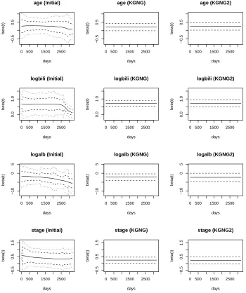
panel: initial estimator in KGNG; Middle panel: KGNG; Right panel: KGNG2. Solid lines: estimated curves; Dashed lines: 95% pointwise confidence inter-vals; Dotted lines: 95% simultaneous confidence bands. . . 27 Figure 2.4 Estimated coefficients for covariates: age, logbili, logalb and stage. Left panel:

initial estimator in KGNG; Middle panel: KGNG; Right panel: KGNG2. Solid lines: estimated curves; Dashed lines: 95% pointwise confidence intervals; Dotted lines: 95% simultaneous confidence bands. . . 28

Figure 3.1 Recurrent event example (CGD data). Top left: ConvexLAR; Top right: vexLASSO; Bottom left: weighted ConvexLAR; Bottom right: weighted Con-vexLASSO. . . 62 Figure 3.2 ConvexLAR and ConvexLASSO solution paths for the panel count data

(bladder) example. . . 64 Figure 3.3 Group LARs solution paths for the Ada-Boost data (WDBC) example. Top

left: GroupConvexLAR-L2; Top right: GroupConvexLAR-L1; Bottom left: GroupConvexLAR; Bottom right: Group ConvexLASSO. . . 67 Figure 3.4 ConvexLAR and ConvexLASSO solution paths for the graphical model (math

score) example. . . 70 Figure 3.5 ConvexLAR and ConvexLASSO solution paths for the graphical model

ex-ample with the simulated data. . . 71

Figure 4.1 The distribution functions of the response Y, in a randomized clinical trial with two treatments,A and B, for male (two panels on the left) and female (two panels on the right). The solid lines with triangle symbol, dashed line, and dotted lines are the conditional mean, 50% quantile, and 25% quantile functions ofY given the gender and the treatment, respectively. . . 79 Figure 4.2 Various loss functions: squared error loss, pinball loss withτ = 0.25, Huber

loss withα= 1 and -insensitive loss with= 1. . . 86 Figure 4.3 Scatterplot and box plots of response Y (CD4 count (cells/mm3) at 20±5

(13)

(14)

Chapter 1

Introduction

As technology advances, massive data sets are collected by human beings in all fields, which

leads to both promises and challenges for researchers. One important issue in analyzing big

volume of data is to find real relationships between the response variable and input covariates

in the data, while getting rid of noisy inputs. Variable/model selection as an useful tool to solve

this problem has received increasing attention in the past few decades. Another interesting topic

is personalized medicine. It is well-known that patients may have heterogeneous responses to

the same treatment or drug. Therefore it would optimize the treatment outcome to develop

individualized treatment for patients. An individualized treatment rule is a rule that assigns a

treatment, from a set of candidate treatments, to a patient according to his/her characteristics,

including genetic, physiological, demographic, environmental, and other clinical information,

and the optimal individualized treatment rule is one such rule which if assigned to the whole

population would lead to the overall “best” outcome. Our main research topic is to find an

efficient and robust way to estimate the optimal individualized treatment rule from the data.

1.1 Variable/Model selection

(15)

elimina-theoretical justification and computational efficiency. In recent years, various modern

vari-able/model selection techniques have been proposed, including but not limited to nonnegative

garrote (Breiman, 1995; Yuan and Lin, 2007), LASSO (Tibshirani, 1996, 1997), SCAD (Fan

and Li, 2001, 2002), adaptive LASSO (Zou, 2006; Zhang and Lu, 2007), group Lasso (Yuan

and Lin, 2006), elastic net (Zou and Hastie, 2005) and MCP (Zhang, 2010). All these methods

can be naturally included in the framework of regularization. Most existing methods focus on

variable selection in the linear model, and less have been studied for nonparametric models or

model structure selection. For example, the identification of linear/nonlinear structure in

par-tially linear regression models or time-invariant/time-varying coefficients in regression models

with time varying coefficients.

In Chapter 2, we explore along this line and study the structure selection problem of

time-varying coefficient Cox models. The time-time-varying coefficient Cox model as a natural extension

of the standard Cox model is widely used to study the temporal effects of covariates. It relaxes

the proportional hazard assumption and can be fitted using either basis expansions (Zucker

and Karr, 1990; Yan and Huang, 2012) or local kernel methods (Cai and Sun, 2003; Tian et al.,

2005). In a time-varying coefficient Cox model, a critical issue is to correctly identify the

mod-el structure, i.e., covariates with null effect, constant effect and truly time-varying effect. By

distinguishing covariates with null effect and non-zero effect, we can build a parsimonious

mod-el with improved risk prediction. By distinguishing covariates with constant effect and truly

time-varying effect, we can build a more interpretable semiparametric model with improved

efficiency over a pure nonparametric model. In this chapter, we will develop a double

penal-ization approach to solve this problem, which also simultaneously estimate the corresponding

regression coefficients.

The majority of existing work conduct model structure selection for the varying coefficient

models by doing hypothesis tests, such as Cai et al. (2000), Huang et al. (2002), Fan and Huang

(2005), Kim (2007), Li and Liang (2008) and Wang et al. (2009), etc. Compared with our

(16)

theoretical justification and computational efficiency. In addition, it is also extremely difficult

to construct a hypothesis test with high power on a large number of covariates simultaneously.

Our proposed methods, KGNG and its variant KGNG2, conduct structure selection and

coefficient estimation simultaneously by coupling the kernel-weighted partial likelihood

esti-mation (Cai and Sun, 2003; Tian et al., 2005) with the group nonnegative garrote penalty.

The performance of our methods is illustrated using simulations and an application to the

primary biliary cirrhosis (PBC) data. Important theoretical properties of the final estimators

are established, including selection consistency, estimation consistency and asymptotic

nor-malities of both the constant coefficients and truly time-varying coefficient functions. Based

on numerical studies, our method can easily handle high dimensional cases with dimension

p over 50. We have developed R code for the proposed methods and make it available at

http://www4.ncsu.edu/~wxiao.

1.2 Computational Issues for High Dimensional Data

Penalized regression is frequently used in high dimensional data analysis. In penalized regression

framework, we usually need to minimize the penalized loss function

M(θ) =L(θ|x) +λP(θ) (1.1)

with respect toθ, whereLis the loss function,P is the penalty andλis the tuning parameter. The tuning parameterλcontrols the magnitude of the penalty, and hence regulates the tradeoffs

between goodness of fit and model sparsity. The performance of penalization methods largely

depends on the choice of the tuning parameter, and careful selection of the tuning parameter is

(17)

computation. First, we can construct a grid points of tuning parameter λand then calculate ˆ

θ(λ) with one value of tuning parameter at a time, using an algorithm such as quadratic programming (QP), the local quadratic approximation (LQA) algorithm (Fan and Li, 2001)

or the local linear approximation (LLA) algorithm (Zou and Li, 2008). To improve the tuning

result, it is essential to make the grid points of tuning parameters finer and finer, which will on

the other hand increase the computation time. This is the main criticism on this type of method.

The second way is to apply a solution path algorithm, which can calculate the minimizer ˆθ(λ) over all values of λ in one shot. Here, we can apply either the approximate path algorithm or the exact path algorithm. One important work in this area is the Least Angle Regression (Efron et al., 2004), which is an extremely efficient exact path algorithm for linear regression.

The Least Angle Regression (LARS) algorithm results in a piecewise solution path, and is

computationally as efficient as Ordinary Least Squares. Rosset and Zhu (2007) derived the

sufficient conditions on the loss and penalty functions, which leads to piecewise linear solution

paths. They have shown that generalized linear models (GLMs) usually do not have piecewise

linear solution paths. Park and Hastie (2006) proposed an approximate path algorithm for

GLMs based on the predictor-corrector method of convex optimization. The algorithm’s overall

accuracy is controlled by a step length parameter. Another approximate path algorithm was

proposed in Friedman (2008) for any convex loss with a separable penalty. Wu (2011) proposed

an ordinary differential equation based exact path algorithm for GLMs, and extended the

algorithm for Cox model considered in Wu (2012). In Chapter 3, we explore along this line and

propose a ConvexLAR algorithm that works for any convex loss function and naturally extends

to group selection and data adaptive variable selection. The algorithm also leads to a new exact

path algorithm for certain penalty methods such as a convex loss function with lasso or group

lasso penalty by a simple modification. We apply the algorithm to various contexts including

recurrent event and panel count data analysis, Ada-Boost, and Gaussian graphical model. The

algorithms are implemented in Matlab and the corresponding code can be downloaded from

(18)

1.3 Optimal Treatment Learning

There is increasing interest to discover individual treatment rules to patients due to their

heterogenous responses to treatment. Here, an individualized treatment rule is a function that

assign a treatment to a patient based on his/her specific characteristics. In particular, we would

like to find an optimal individualized treatment rule, which if applied to the whole population

would lead to the “best” outcome. For complex diseases such as cancer and AIDS, the optimal

individualized treatment rule is usually a dynamic treatment process, which involves a sequence

decisions over the time. In this case, we also name it dynamic treatment regimes.

Q-learning (Watkins and Dayan, 1992; Murphy, 2005) and A-learning (Murphy, 2003;

Robin-s, 2004) are two main approaches for estimating optimal dynamic treatment regimes. Q-learning

is based on posing a regression model to estimate the conditional expectation of the outcome

at each time point, and then applying a backward recursive procedure to fit the model.

A-learning, on the other hand, only requires modeling the contrast function of the treatments

at each time point, and it is therefore more flexible and robust to a model misspecification.

Alternative methods include regret regression (Henderson et al., 2010) and direct value

max-imization (Zhao et al., 2012; Zhang et al., 2013). Specifically, Zhao et al. (2012) proposed an

outcome weighted learning approach using a surrogate loss to approximate a 0-1 loss, and the

approach is based on support vector machine framework. Zhang et al. (2013) estimates the

dy-namic treatment regime by maximizing a doubly robust augmented inverse probability weighted

estimator for mean outcome over a restricted class of regimes. The method proposed in Zhang

et al. (2013) is robust against model misspecification, but computational intractable when the

restricted class of regimes are in high dimension setting.

Variable selection is important to estimate optimal individualized treatment rule in high

dimensional data analysis. Related work includes Qian and Murphy (2011) and Lu et al. (2013).

The former one employs a flexible model estimation framework to approximate the conditional

(19)

In Chapter 4, we will develop new estimators for optimal individualized treatment rules

via robust regression. Compared with standard Q- and A-learning, which both mimic a least

squares regression, our new estimators are robust against the skewed, heterogeneous,

heavy-tailed errors or outliers. Furthermore, the new estimators are robust against misspecification of

the baseline function, which is a nice property shared by A-learning. Last but not least, under

certain situations, i.e. when the error term is interacted with the treatment, the new estimator

coupled with pinball loss approximately maximizes the outcomes conditional quantile instead

of conditional mean, which leads to a different optimal individualized treatment rule from

the traditional Q- and A-learning. We demonstrate the performance of the new estimators by

(20)

Chapter 2

Joint Structure Selection and

Estimation in the Time-varying

Coefficient Cox Model

2.1 Introduction

Cox proportional hazards model (Cox, 1972) has become the most popularly used

semiparamet-ric model in survival analysis due to its nice hazard interpretation and easy estimation based on

partial likelihood principle with elegant counting process-based martingale theory (Andersen

and Gill, 1982). However, one main limitation of the standard Cox model is to assume that the

hazard ratios stay constant over time, i.e. covariate effects are time-invariant, which may be

unrealistic in practical applications. Many alternatives have been proposed to relax the

propor-tional hazards assumption. Among them, the time-varying coefficient Cox model is a natural

extension of the standard Cox model by allowing temporal effects of covariates, and has been

widely studied in the literature (e.g. Zucker and Karr, 1990; Cai and Sun, 2003; Tian et al.,

(21)

model structure, i.e. to distinguish covariates with null effect, constant effect or truly

time-varying effect. There are at least two benefits. On one hand, by identifying covariates with null

effect and excluding them from the model, we can build a parsimonious model with better risk

prediction. On the other hand, by distinguishing covariates with constant effect and truly-time

varying effects, we can build a simpler and easier-interpretable semiparametric model comparing

with a pure nonparametric model with time-varying coefficients, which will be highly

appre-ciated by empirical investigators since they generally prefer a flexible but easy-interpretable

model for data analysis. See Zhang et al. (2002); Fan and Huang (2005); Ahmad et al. (2005);

Wang et al. (2009) for more demonstration of the benefits of semiparametric varying-coefficient

models comparing with nonparametric varying-coefficient models.

Model selection has been extensively studied in the past few decades. Traditional model

se-lection techniques, such as best-subset sese-lection, coupled withCp (Mallows, 1973), AIC (Akaike, 1973) and BIC (Schwarz, 1978), separate model selection and model estimation steps and are

generally unstable due to the their inherent discreteness (Breiman, 1995) and stochastic errors

(Fan and Li, 2001). They also lack of asymptotic selection consistency, which is a desirable

asymptotic property to possess. More importantly, they are not computational feasible for data

set with moderate to large dimensions as their computation times increase exponentially with

the dimension. To overcome these difficulties, various penalization methods have been

intro-duced, for example, nonnegative garrote (Breiman, 1995), LASSO (Tibshirani, 1996, 1997),

SCAD (Fan and Li, 2001, 2002) and adaptive LASSO (Zou, 2006; Zhang and Lu, 2007). These

methods provide competing performance for simultaneously selecting important variables and

estimating their effects. However, most existing penalization methods focus on variable

selec-tion for simple linear regression models. Less has been studied for model structure selecselec-tion,

for example, the identification of linear/nonlinear structure in partially linear regression models

or time-invariant/time-varying coefficients in regression models with time-varying coefficients.

Recently, Zhang et al. (2011) proposed a novel penalization approach in the frame of

(22)

nonlinear effect in a partially linear model. For censored data, Yan and Huang (2012) proposed

an adaptive group LASSO (AGLASSO) method based on a penalized B-spline approach for

model structure selection in a time-varying coefficient Cox model. Specifically, time-varying

coefficients are expanded with a set of B-spline basis functions and an adaptive group lasso

penalty is used to select between time-independent and time-dependent covariate effects.

In this chapter, we propose an alternative method for automatic model structure

selec-tion and coefficient estimaselec-tion in a time-varying coefficient Cox model by coupling the

kernel-weighted partial likelihood estimation (Cai and Sun, 2003; Tian et al., 2005) with the group

nonnegative garrote penalty. There are three major motivations for developing this new

ap-proach based on local kernel methods. First, in contrast with the spline method proposed in

Yan and Huang (2012), our method is able to better capture some local features of time-varying

coefficient functions, which are otherwise hard to be captured by the spline method. Second, by

using the local kernel estimation, it enables us to rigorously study the asymptotic properties of

the proposed estimators for both constant and time-varying coefficients, such as model

selec-tion consistency and asymptotic normality, and hence justify the validity of the methods from

theoretical perspectives. None of these properties have been established for existing approaches

like Yan and Huang (2012). Third, the proposed method provides an automatic and effective

way to conduct structure selection for time-varying coefficient Cox model, which can deal with

relative large dimension in contrast with all existing methods based on hypothesis testing, such

as those studied in Tian et al. (2005) and Liu et al. (2013). The remainder of the chapter is

organized as follows. Our proposed kernel group nonnegative garrote (KGNG) method and its

variant (KGNG2) are introduced in Section 2.2. Asymptotic properties of KGNG and KGNG2

estimators are presented in Section 2.3. Section 2.4 is devoted to numerical studies, including

simulations and an application to the primary biliary cirrhosis data. All the technical proofs

(23)

2.2 Structure Selection with Kernel Group Nonnegative

Gar-rote

2.2.1 Methods

Consider a random sample of n individuals. Let Ti be the failure time, Ci be the censoring time, andZi be ap-vector of covariates for subjecti. Conditional onZi,Ti andCi are assumed independent. Define Te_i = min(T_i, C_i) and ∆_i = 1(T_i ≤ C_i). The data consist of the triplets (Te_i,Zi,∆_i),i= 1, . . . , n. The time-varying coefficient Cox model assumes the following form

α(t|Z_i) =α0(t)eβ

T

0(t)Zi, (2.1)

where α(·|Zi) is the conditional hazard function given covariates, α0(·) is a completely un-specified baseline hazard function, andβ₀(t) = (β01(t), . . . , β0p(t))T is a p-dimensional smooth function of t.

Without loss of generality, we assumeβ₀(t) = (βT

O(t),β

T

C(t),β

T

N C(t))T, whereβO(t)∈IRp1, β_C(t) ∈IRp2 _and _β

N C(t) ∈IRp3 correspond to covariates with null effect, constant effect and truly time-varying effect, respectively, and p = p1 +p2+p3. Denote the corresponding index

sets of the above three classes by IO, IC and IN C, and let I = {1, . . . , p} = {IO S

IC S

IN C}. Our method consists of two steps. In Step 1, for any fixed t, we obtain the initial estimator

e

β(t) = (β1e(t), . . . ,βe_p(t))T ∈ IRp using the kernel-weighted partial likelihood estimation (Cai and Sun, 2003; Tian et al., 2005), i.e., by maximizing the local partial likelihood

L1n(β, t) = 1

n

n X

i=1

Z τ

0

Kh(s−t) 

β

T_Z

i−log 

 n X

j=1

Yj(s)eβ

T Zj



 

dNi(s), (2.2)

(24)

into the mean partfm= (m1, . . . ,e mep)

T_{and the deviation part}

e

β∗(t) = (βe₁∗(t), . . . ,βe_p∗(t))T, where

e

mk =τ−1 Rτ

0 βe_k(u)duand βe∗_k(t) =βe_k(t)−m_e_k for k= 1, . . . , p. Practically, we could chooseM grid points T_M = {t1, . . . , tM}, equally spaced between 0 and τ, where M is a large positive integer. We then let m_ek =PMi=1βe_k(t_i)/M and βe_k∗(t) =βe_k(t_j)−m_e_k, wherej = argmin_k|t_k−t| and t∈[0, τ]. In our numerical studies, we setM to be 100, which based on our experiment is large enough to make good approximation of both m_ek and βe_k∗(t).

In Step 2, we adapt group nonnegative garrote penalties for structure selection. Denote

λ1 = (λ11, . . . , λ1p)T,λ2 = (λ21, . . . , λ2p)T as two p-dimensional vectors. We obtain λb₁ and λb₂ by minimizing

Q2n(λ1,λ2) =−

n X

i=1

Z τ

0

"

f

m◦λ1+βe

∗

(s)◦λ2

T

Zi

−log 

 n X

j=1 Yj(s)e

f m◦λ1+βe

∗

(s)◦λ2 T

Zj



 #

dNi(s)

+θ1

p X

j=1

λ1j+θ2

p X

j=1

λ2j (2.3)

subject toλ1j ≥0 andλ2j ≥0,j= 1,· · · , p, whereθ= (θ1,θ2) are two-dimensional nonnegative

tuning parameters, anda◦b denotes the Hadamard (element-wise) product of vectorsaandb. Then, the proposed KGNG estimator ofβ0k(t) is given by

b

βk(t) =bλ1_km_e_k+bλ2_kβe_k∗(t), k= 1, . . . , p, t∈[0, τ]. (2.4)

It is interesting to note that the automatic structure selection is achieved by shrinking some

components of λb₁ and λb₂ to zero. Specifically, we definebI_O = {k ∈ I : λb₁_k = 0,bλ₂_k = 0},

bI_C ={k∈I :bλ₁_k6= 0,λb₂_k = 0}andbI_{N C} ={k∈I :λb₂_k6= 0} as estimated index sets for I_O, I_C and IN C, respectively.

(25)

variant of KGNG estimator. Specifically, we add a preliminary step (Step 0) before Steps 1 and

2 to exclude all noise variables prior to structure selection. To do this, we conduct a standard

group nonnegative garrote estimation by minimizing

Q0n(λ∗) =− n X i=1 Z τ 0   e

β(s)◦λ∗ T

Zi−log 

 n X

j=1 Yj(s)e

e

β(s)◦λ∗ T

Zj



 

dNi(s)

+θ∗

p X

j=1

λ∗_j (2.5)

with respect to λ∗ = (λ∗₁, . . . , λ∗_p)T_{, where}_λ∗

j ≥0,j = 1, . . . , p, and θ∗ is a nonnegative tuning parameter. Letλb

∗

= (bλ∗₁, . . . ,bλ∗_p)Tdenote the resulting minimizer. We exclude thekth covariate if bλ∗_k = 0. Let Z_i denote the remaining sub-vector of Zi by keeping all important covariates. We then implement Steps 1 and 2 withZi replaced by Z_i for further structure selection. The resulting estimator is denoted as KGNG2.

2.2.2 Computational Aspects

We implemented the proposed method in R, and the corresponding code can be

download-ed from the author’s web page (http://www4.ncsu.edu/sim/wxiao/). In Step 1, L1n(β, t) is strictly concave with probability one and thus has a unique solution. The maximization can be

realized based on a regular Newton-Raphson iteration or an efficient iterative algorithm

pro-posed in Cai et al. (2000). In Step 2, after proper transformations, the minimization problem of

(2.3) is equivalent to finding the lasso solution for a Cox model with time-dependent covariates

e

Zi(s) under the nonnegative constraint of regression parameters, where

e Zi(s) =



 

f m◦Zi

e

β∗(s)◦Zi 

 .

We used R package “penalized” (Goeman, 2010) for this optimization step. The algorithm is

(26)

can also incorporate nonnegative constraints on the parameters (Goeman, 2010). Moreover, the

minimization in the preliminary Step 0 is also equivalent to finding a lasso solution for a Cox

model with time-dependent covariates βe(s)◦Zi. Therefore it can be computed similarly with existing R packages.

2.2.3 Tuning Procedure

For computing KGNG, two sets of tuning parameters need to be chosen properly, i.e., the

bandwidth h at the maximum local partial likelihood estimation step (2.2) and (θ1, θ2) at the

group nonnegative garrote estimation step (2.3). To chooseh, we use a K-fold cross-validation

method as suggested in Tian et al. (2005). First, we randomly split the data set intoK roughly equal-sized parts. Then, for each k= 1, . . . , K, we delete the kth part and fit the time-varying

coefficient Cox model with the otherK−1 parts. Next, we compute the prediction errorP Ek(h), which measures how well the fitted model predicts the kth part of the data. Here,

P Ek(h) =− X

i∈Ik

Z τ

0



 bβ

(−k)

(s)T

Zi−log 

 X

j∈Ik

Yj(s)e

b

β(−k)(s)T_Z j



 

dN_i(s),

where Ikis the index set for the kth part of the data andβb

(−k)

(t) is the maximum local partial

likelihood estimator calculated with the kth part of the data deleted. Last, the optimal h is

obtained by minimizing the total prediction errorP E(h) =PK

k=1P Ek(h).

For (θ1, θ2), we consider a set of bivariate grid values, and choose the optimal (θ1, θ2) by minimizing the following BIC criterion

BIC=−2 log(partial likelihood)/n+ logn/n×df1+ log(nh∗)/(nh∗)×df2,

where df1 and df2 are the number of nonzero components in λb₁ and λb₂, respectively, and

h∗ =h/τ is the effective bandwidth when we scale τ to 1. Note that the effective sample size

(27)

fact thatβ∗_i(t) is estimated locally. Similar strategy is adopted in Wang and Xia (2009) and Hu and Xia (2012).

Similarly, θ∗ in the preliminary Step 0 can be chosen by minimizing the BIC criterion

BIC=−2 log(partial likelihood)/n+ log(nh∗)/(nh∗)×df3,

wheredf3 is the number of covariates with nonzero effect.

2.3 Theoretical properties

In this section, we establish the asymptotic properties of the initial estimators, and our proposed

KGNG and KGNG2 estimators.

2.3.1 Asymptotic Properties of Initial Estimators

Denote the true mean and deviation part of β₀(t) as m0 = (m01, . . . , m0p)T and β∗0(t) =

(β∗₀₁(t), . . . , β₀∗_p(t))T_{, respectively, where}

m0k=τ−1 Z τ

0

β0k(u)du, β0∗k(t) =β0k(t)−m0k,

fork= 1, . . . , p. LetI(β, t) =−∂2L1n(β, t)/∂β2 =n−1 Pn

i=1

Rτ

0 V(β, s)Khn(s−t)dNi(s), where

V(β, t) =S

(2)₍_β_{, t}₎ S(0)₍_β_{, t}₎ −

S(1)₍_β_{, t}₎ S(0)₍_β_{, t}₎

!⊗2

,

S(r)(β, t) =n−1

n X

i=1

Yi(t)Zi⊗reβ

0

Zi_{, r}_{= 0}_,₁_,₂_,

with⊗ denoting the outer product. LetE(β, t) =S(1)₍_β_{, t}₎_/S(0)₍_β_{, t}_),_P₍_t_|z_{) = P(}

e

T ≥t|Z= z), Q0(t) = E[P(t|Z)α(t|Z)], Q1(t) = E[P(t|Z)α(t|Z)Z] and Q2(t) = E[P(t|Z)α(t|Z)Z⊗2].

Define Σ(t) =Q2(t)−Q1(t)Q1(t)T/Q0(t). Lets(r)(β, t) denote the limits ofS(r)(β, t),r= 0,1,2,

(28)

set of IRp that includes a neighborhood of β₀(t) for t ∈ [0, τ]. Under the following regularity conditions,

(A.1) The kernel functionK(·) is a bounded and symmetric density with a bounded support [-1,1];

(A.2) Fort∈[0, τ]

E "

exp (

2 sup

u∈N(t,)

|β₀(u)|+β0₀(t) + 3 !

|Z| )#

<∞;

(A.3) Q0(u)>0,Q1(u) andQ2(u) are continuous fort∈[0, τ];

(A.4) Assume that α0(t) is positive and continuous, P(t|z) > 0 and coefficient functions {β0j(t)} have a continuous second derivative fort∈[0, τ];

(A.5) Assume that the matrix Σ(t) is positive definite fort∈[0, τ];

(A.6) s(r)(β, t) is uniformly continuous with respect to (βT_{, t}₎T_{∈ B ×}_[0_{, τ}_{] for}_t_∈_[0_{, τ}_];

we have

Lemma 2.1. Suppose hn=O(n−ν) with ν ∈[1/5,1).

(a) βe(t) p

→β₀(t), 0≤t≤τ.

(b) If 1/5< ν <1, we have, for fixedt∈(0, τ),

(nhn)1/2

e

β(t)−β₀(t) _d

→N

0, Σ−1(t) Z 1

−1

K2(s)ds

.

where Σ(t) can be consistently estimated byI(eβ(t), t).

(29)

where Σm = Rτ

0 Σ

−1₍_u₎_du/τ2 _{and can be consistently estimated by}

b Σm=

Z τ−h h

I−1(βe(u), u)du/(τ−2h)2.

The proof of Lemma 2.1 follows Cai and Sun (2003) which is omitted. The proof of

Lem-ma 2.2 follows similar steps given in Section 5 of Tian et al. (2005) and is relegated to the

Supplement.

2.3.2 Asymptotic Properties of KGNG Estimators

Letλ01andλ02denote the true values ofλ1 andλ2, respectively, and partition them into three

parts: λ01= (λO01

T

,λC₀₁T,λN C₀₁ T)T _{and (}_λO

02

T

,λC₀₂T,λN C₀₂ T)T_{, according to the true index sets I}

O, IC and IN C, respectively. Then

λO₀₁=0p1, λ

C

01=1p2, λ

O

02=0p1, λ

C

02=0p2, λ

N C

02 =1p3

andλN C₀₁_,j = 0 or 1 forj∈IN C, whereλN C01,j is thejth component ofλN C01 and corresponds to the

mean part of thejth covariate with time-varying effect. IfλN C₀₁_,j = 0, thejth time-varying effect has zero mean effect; otherwise, it has nonzero mean effect. As we do not distinguish between

the above two types of time-varying effects, without loss of generality, we assumeλN C₀₁ =1p3 in

our theoretical derivations. Let λ0 = (λT01,λ02T )T. We further partition λ0 asλ(1)0 representing

all the ones and λ(0)₀ representing all the zeros, where λ(1)₀ = (λC₀₁T,λN C₀₁ T,λN C₀₂ T)T ₌ ₁

p2+2p3

and λ(0)₀ = (λO₀₁T,λO₀₂T,λC₀₂T)T ₌ ₀

2p1+p2. In a similar manner we define λ, λ

(1)_,_λ(0)_,

b λ, λb

(1)

and λb

(0)

, which accord to the true index sets IO, IC and IN C.

Note that the KGNG estimator defined in (2.4) takes the form βb(t) =λb₁◦_fm+λb₂◦βe

∗

(t).

To derive its asymptotic properties, we need to study the asymptotic properties of fm, βe

∗

(t)

and λb. In Lemmas 2.1 and 2.2, we have established the asymptotic properties ofm_f andβe

∗

(t). In the following, we derive the asymptotic properties of λb, which consists ofλb

(1)

and λb

(0)

. In

particular, we establish the root-n consistency ofλb

(1)

(30)

of λb

(0)

in Theorem 2.2.

Theorem 2.1. Assume hn = O(n−ν) with 1/4 < ν < 1/2. Under the regularity conditions

assumed in Lemmas 2.1 and 2.2, ifmax(θ1, θ2)/√nis bounded, thenkλb

(1)

−λ(1)₀ k=Op(n−1/2). Theorem 2.2. Assume hn = O(n−ν) with 1/4 < ν < 1/2. Under the regularity conditions

assumed in Lemmas 2.1 and 2.2, if kλb

(1)

−λ(1)₀ k=Op(n−1/2) andh1n/2min (θ1, θ2)→ ∞, then P(λb

(0)

=0)→1.

Combining Theorems 2.1 and 2.2, we can then prove the selection consistency of the KGNG

estimator, which is summarized in part (a) of Theorem 2.3. We further establish the

asymp-totic normality of the KGNG estimators for both nonzero constant and time-varying regression

coefficients in Theorem 2.3. Recall that β₀(t) = (βT

O,β

T

C,β

T

N C(t))T ∈ IRp, where βO ∈ IRp1, β_C ∈IRp2 _and _β

N C(t)∈IRp3 are subvector ofβ0(t) corresponding to the true underline index

sets IO, IC and IN C, respectively. In a similar manner, we write m0 = (mTO,m

T

C,m

T

N C)

T _and

β∗₀(t) = (β∗_OT

,β∗_CT

,β∗_{N C}T

(t))T_{. We further partition}

b

β(t), βe(t), f mand βe

∗

(t) accordingly.

assumed in Lemmas 1 and 2, if max(θ1, θ2)/√n is bounded and hn1/2min (θ1, θ2)→ ∞, then

(a) (Selection consistency) with probability tending to one,bI_O = I_O,bI_C = I_C andbI_{N C} =

IN C.

(b) (Root-n consistency of βb_C) βb_C is a root-n consistent estimator for β_C.

(c) (Asymptotic normality of βb_C) if we further assume max(θ1, θ2)/

√

n→0,

(n)1/2βb_C−β_C _d

→N

0, ΣF_m ,

where

ΣF_m = Z τ

0

D(u) +1

τB10Σ

−1₍_u₎

Σ(u)

D(u) +1

τB10Σ

−1₍_u₎

T

(31)

(d) (Asymptotic normality of βb_{N C}(t))

(nhn)1/2

b

β_{N C}(t)−β_{N C}(t) _d

→N

0, {Σ−1(t)}N C,N C Z 1

−1

K2(s)ds

,

where {Σ−1(t)}_{N C,N C} is the submatrix of Σ−1(t) corresponding to IN C.

The proofs of Theorem 2.1, 2.2 and 2.3 are relegated to the Supplement. The asymptotic

variance-covariance matrices given in parts (c) and (d) can be consistently estimated by the

usu-al plug-in method. It is interesting to note that the limiting distribution of the KGNG estimator

for the time-varying coefficients given in part (d) is the same as that of the corresponding initial

estimator. Actually in the proof of part (d), we have shown that the difference betweenβb_{N C}(t) and βe_{N C}(t) are uniformly asymptotically negligible in t. Thus we could construct confidence bands ofβb_{N C}(t) using the resampling technique as proposed in Tian et al. (2005).

2.3.3 Asymptotic Properties of KGNG2 Estimator Let Z = (ZT

O,ZCT,ZN CT )T and Z = (ZCT,ZN CT )T as the subvector of Z with only important covariates kept. Letβ

0(t) = (β

T

C(t),βTN C(t))T,α(t|Z) =α0(t)eβ0(t) T_Z

,P(t|Z) =P(Y ≥t|Z= z), Q₀(t) = E[P(t|Z)α(t|Z)], Q₁(t) = E[P(t|Z)α(t|Z)Z] and Q₂(t) = E[P(t|Z)α(t|Z)Z⊗2]. Define Σ(t) = Q₂(t)−Q₁(t)Q₁(t)T_/Q

0(t). We add “*” to distinguish the KGNG2 estimator

from the KGNG estimator. We summarize the asymptotic properties of KGNG2 estimator in

Theorem 2.4.

assumed in Lemmas 1 and 2, if (1)θ∗/√n is bounded andhn1/2θ∗→ ∞; (2)max(θ1, θ2)/ √

nis bounded and h1n/2min (θ1, θ2)→ ∞, then

(a) (Selection consistency of preliminary Step 0)with probability tending to one,bλ∗_k = 0,

for k∈IO and bλ∗_k6= 0, for k∈I_C S

IN C.

(b) (Selection consistency) with probability tending to one,bI∗_O = I_O,bI∗_C = I_C andbI∗_{N C} =

(32)

(c) (Root-n consistency of βb

∗

C) βb

∗

C(t) is a root-n consistent estimator for βC.

(d) (Asymptotic normality of βb

∗

C) if we further assume max(θ1, θ2)/ √

n→0,

(n)1/2βb

∗

C−βC _d

→N

0, ΣF_m ,

where ΣF_m can be computed following (2.6)with some obvious changes.

(e) (Asymptotic normality of βb

∗

N C(t))

(nhn)1/2

b

β∗_{N C}(t)−β_{N C}(t) _d

→N

0, {Σ−1(t)}N C,N C Z 1

−1

K2(s)ds

,

where {Σ−1(t)}_{N C,N C} is the submatrix of Σ−1(t) corresponding to IN C.

The proof of Theorem 2.4 is similar to that of Theorem 2.3 and hence is omitted here.

Based on Theorem 2.3 and 2.4,βb

∗

N C(t) is strictly more efficient thanβb_{N C}(t) if I_Ois not empty. However, there is no clear order between the efficiencies of βb

∗

C and βb_C.

2.4 Numerical studies

2.4.1 Simulation studies

We generate failure times from the varying-coefficient Cox model (2.1). Here, covariate vectorZ is generated from a multivariate normal distribution with mean 0, variance 0.5 and correlation

coefficient 0.5|j−k|for any pair (j, k). We consider both the low dimensional case and the high dimensional case, where the dimension p = 10 and 50 respectively. There are three nonzero

coefficients in β₀(t), i.e., β02(t) = −{1 + cos(πt)}1(0 < t < 1), β03(t) = 1.5{cos(πt/2)} and

β08(t) =−1. So, there are two covariates with time-varying effects, one with constant effect and

all the remains with null effect. The baseline hazard function α0(t) = exp{−cos(πt/2)}. We

(33)

ith subject is a mixture ofW and a point mass at 2, whereW = min(exp(Zi2−Zi5), Unif(0,2)).

When p = 50, we generate censoring times from a mixture of Unif(0,2)) and a point mass at

2. For both cases, the mixing probability is chosen to have the desired censoring proportion,

i.e. cp = 20% or 40%. For each scenario, we conduct 100 simulation runs with sample size

n= 200 and 400. We compare the proposed KGNG and KGNG2 with the AGLASSO of Yan

and Huang (2012). For our estimators, we use the Epanechnikov kernel K(x) = 3(1−x2)/4, −1 ≤ x ≤ 1. The bandwidth h is chosen using 5-fold cross validation as discussed in Section 2.2.3. For KGNG2, the same bandwidth is used for Step 1 as for Step 0. We use the proposed

BIC criterion in Section 2.2.3 to tune (θ1, θ2) and θ∗.

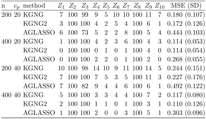
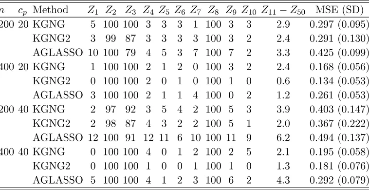
Tables 2.1 and 2.2 summarize the mean squared errors and variable selection results for

p= 10 and 50, respectively. The selection frequency of each variable over 100 runs is reported,

where the important covariates areZ2,Z3 andZ8. The mean squared error (MSE) is calculated

as

1 100

100

X

i=1

n b

β(ti)−β0(ti) oT

V

n b

β(ti)−β0(ti) o

,

where {t1, . . . , t100} are 100 equally-spaced grid points in the time interval (0,2) andV is the

population covariance matrix of covariates.

From Tables 2.1 and 2.2, we make the following observations. First, KGNG2 shows the

best performance in terms of variable selection and MSE in almost all scenarios, especially for

large dimension case (p= 50). This is expected since KGNG2 is a two-stage approach, by first

excluding the noise variables. Second, both KGNG and KGNG2 outperform AGLASSO with

deduction in MSE as large as 60%. Third, KGNG and KGNG2 selectZ2,Z3andZ8as important

covariates nearly all the times, while the AGLASSO missesZ3occasionally, especially when the sample size is small.

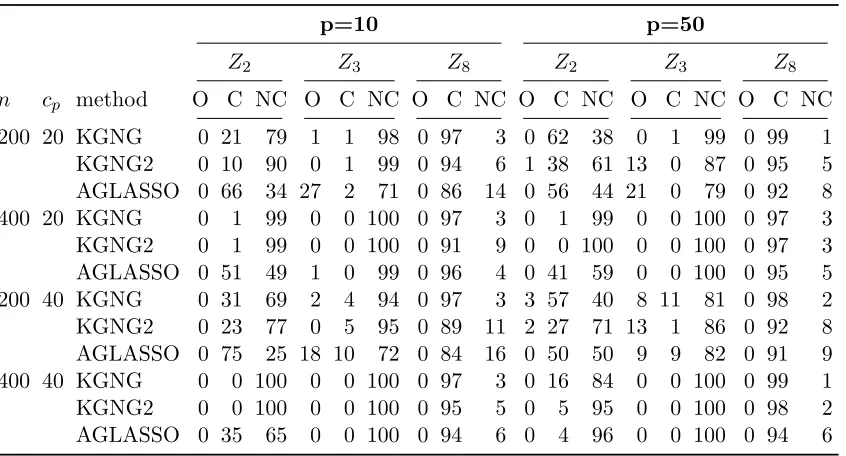
Table 2.3 summarizes the structure selection result of the three covariates with nonzero

(34)

Table 2.1: Variable selection and estimation results forp= 10. MSE stands for mean-squared error. Standard deviations of the Monte Carlo estimates are given in parentheses.

n cp method Z1 Z2 Z3 Z4 Z5 Z6 Z7 Z8 Z9 Z10 MSE (SD)

200 20 KGNG 7 100 99 9 5 10 10 100 11 7 0.180 (0.107) KGNG2 3 100 100 4 2 5 4 100 6 1 0.172 (0.126) AGLASSO 6 100 73 5 2 2 8 100 5 4 0.444 (0.103) 400 20 KGNG 1 100 100 4 2 3 6 100 4 3 0.114 (0.053) KGNG2 0 100 100 0 1 0 1 100 4 0 0.114 (0.054) AGLASSO 0 100 100 2 2 0 1 100 2 0 0.268 (0.055) 200 40 KGNG 10 100 98 14 10 9 11 100 14 5 0.244 (0.151) KGNG2 7 100 100 7 5 3 5 100 11 3 0.227 (0.176) AGLASSO 7 100 82 9 4 4 6 100 6 1 0.492 (0.122) 400 40 KGNG 5 100 100 3 3 4 4 100 7 2 0.117 (0.080) KGNG2 2 100 100 1 1 0 1 100 3 1 0.110 (0.126) AGLASSO 1 100 100 2 0 0 3 100 5 1 0.303 (0.096)

select the time-varying-effect Z2 as a constant-effect covariate. For example, when p = 10,

n= 200 and cp = 20%, AGLASSO correctly classifies Z2 only 34 times out of 100, while both

KGNG and KGNG2 classify Z2 correctly for more than 70 times.

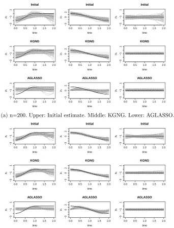
Finally, we plot the initial estimator, KGNG and AGLASSO for three nonzero coefficients

and their pointwise 95% confidence intervals based on 100 simulations for p = 10. The plots

forcp = 20% andcp = 40% are given in Figures 2.1 and 2.2, respectively. We make the follow-ing observations. First, the performance of both KGNG and AGLASSO improves substantially

when sample size increases. Second, KGNG has smaller biases in the estimation of time-varying

coefficients compared with AGLASSO in all the cases, while KGNG and AGLASSO give

com-parable estimates for the constant coefficient. Third, the improvement of KGNG over the initial

estimator for time-varying coefficients is not obvious, however, the improvement for the constant

(35)

0.0 0.5 1.0 1.5 2.0 −3 −1 1 Initial time β2

0.0 0.5 1.0 1.5 2.0

−3 0 2 Initial time β3

0.0 0.5 1.0 1.5 2.0

−3 −1 1 Initial time β8

0.0 0.5 1.0 1.5 2.0

−3 −1 1 KGNG time β2

0.0 0.5 1.0 1.5 2.0

−3 0 2 KGNG time β3

0.0 0.5 1.0 1.5 2.0

−3 −1 1 KGNG time β8

0.0 0.5 1.0 1.5 2.0

−3 −1 1 AGLASSO time β2

0.0 0.5 1.0 1.5 2.0

−3 0 2 AGLASSO time β3

0.0 0.5 1.0 1.5 2.0

(a) n=200. Upper: Initial estimate. Middle: KGNG. Lower: AGLASSO.

0.0 0.5 1.0 1.5 2.0

−3 −1 1 KGNG time β2

0.0 0.5 1.0 1.5 2.0

−3 0 2 KGNG time β3

0.0 0.5 1.0 1.5 2.0

−3 −1 1 KGNG time β8

0.0 0.5 1.0 1.5 2.0

(b) n=400. Upper: Initial estimate. Middle: KGNG. Lower: AGLASSO.

Figure 2.1: Estimated curves (gray) of the three nonzero coefficients from 100 replicates when

(36)

0.0 0.5 1.0 1.5 2.0 −3 −1 1 Initial time β2

0.0 0.5 1.0 1.5 2.0

−3 −1 1 KGNG time β2

0.0 0.5 1.0 1.5 2.0

−3 0 2 KGNG time β3

0.0 0.5 1.0 1.5 2.0

−3 −1 1 KGNG time β8

0.0 0.5 1.0 1.5 2.0

(a) n=200. Upper: Initial estimate. Middle: KGNG. Lower: AGLASSO.

0.0 0.5 1.0 1.5 2.0

−3 −1 1 KGNG time β2

0.0 0.5 1.0 1.5 2.0

−3 0 2 KGNG time β3

0.0 0.5 1.0 1.5 2.0

−3 −1 1 KGNG time β8

0.0 0.5 1.0 1.5 2.0

(b) n=400. Upper: Initial estimate. Middle: KGNG. Lower: AGLASSO.

Figure 2.2: Estimated curves (gray) of the three nonzero coefficients from 100 replicates when

(37)

Table 2.2: Variable selection and estimation results forp= 50. MSE stands for mean-squared error. Standard deviations of the Monte Carlo estimates are given in parentheses.

n cp Method Z1 Z2 Z3 Z4 Z5 Z6 Z7 Z8 Z9 Z10 Z11−Z50 MSE (SD)

200 20 KGNG 5 100 100 3 3 3 1 100 3 3 2.9 0.297 (0.095) KGNG2 3 99 87 3 3 3 3 100 3 2 2.4 0.291 (0.130) AGLASSO 10 100 79 4 5 3 7 100 7 2 3.3 0.425 (0.099) 400 20 KGNG 1 100 100 2 1 2 0 100 3 2 2.4 0.168 (0.056) KGNG2 0 100 100 2 0 1 0 100 1 0 0.6 0.134 (0.053) AGLASSO 3 100 100 2 1 1 4 100 0 2 1.2 0.261 (0.053) 200 40 KGNG 2 97 92 3 5 4 2 100 5 3 3.9 0.403 (0.147) KGNG2 2 98 87 4 3 2 2 100 5 1 2.0 0.367 (0.222) AGLASSO 12 100 91 12 11 6 10 100 11 9 6.2 0.494 (0.137) 400 40 KGNG 0 100 100 4 0 1 2 100 2 5 2.1 0.195 (0.058) KGNG2 0 100 100 1 0 0 1 100 1 0 1.3 0.181 (0.076) AGLASSO 5 100 100 4 1 2 3 100 6 2 4.3 0.292 (0.079)

2.4.2 Analysis of primary biliary cirrhosis (PBC) data

As an illustration, we apply our KGNG and KGNG2 methods to analyze the PBC data

(Flem-ing and Harr(Flem-ington, 1991). The data is from the Mayo Clinic trial in primary biliary cirrhosis

(PBC) of the liver conducted between 1974 and 1984. The primary biliary cirrhosis is a chronic

disease in which the bile ducts in one’s liver are slowly destroyed. In the study, 312 out of 424

patients who participate in the randomized trial are eligible for the analysis. There are 17

co-variates: trtmt=treatment (Yes/No), age (in 10 years), gender=female/male, ascites=presence

of ascites (Yes/No), hypato=presence of hepatomegaly (Yes/No), spiders=presence of

spider-s, edema=severity of oedema (0 denotes no oedema, 0.5 denotes untreated or successfully

treated oedema and 1 denotes unsuccessfully treated oedema), logbili=logarithm of serum

bilirubin (mg/dl), chol=serum cholesterol (mg/dl), logalb=logarithm of albumin (gm/dl),

cop-per=urine copper (mg/day), alk=alkaline phosphatase (U/liter), sgot=liver enzyme (U/ml),

trig=triglicerides (mg/dl), platelet=platelets per 10−3ml3, logprotime=logarithm of

prothrom-bin time (seconds), stage=histologic stage of disease (category: 1, 2, 3 or 4).

(38)

Table 2.3: Structure selection results for covariates 2, 3 and 8. Here O is for null effect, C for constant effect, and NC for time-varying effect.

p=10 p=50

Z2 Z3 Z8 Z2 Z3 Z8

n cp method O C NC O C NC O C NC O C NC O C NC O C NC

200 20 KGNG 0 21 79 1 1 98 0 97 3 0 62 38 0 1 99 0 99 1

KGNG2 0 10 90 0 1 99 0 94 6 1 38 61 13 0 87 0 95 5

AGLASSO 0 66 34 27 2 71 0 86 14 0 56 44 21 0 79 0 92 8

400 20 KGNG 0 1 99 0 0 100 0 97 3 0 1 99 0 0 100 0 97 3

KGNG2 0 1 99 0 0 100 0 91 9 0 0 100 0 0 100 0 97 3

AGLASSO 0 51 49 1 0 99 0 96 4 0 41 59 0 0 100 0 95 5

200 40 KGNG 0 31 69 2 4 94 0 97 3 3 57 40 8 11 81 0 98 2

KGNG2 0 23 77 0 5 95 0 89 11 2 27 71 13 1 86 0 92 8

AGLASSO 0 75 25 18 10 72 0 84 16 0 50 50 9 9 82 0 91 9 400 40 KGNG 0 0 100 0 0 100 0 97 3 0 16 84 0 0 100 0 99 1

KGNG2 0 0 100 0 0 100 0 95 5 0 5 95 0 0 100 0 98 2

AGLASSO 0 35 65 0 0 100 0 94 6 0 4 96 0 0 100 0 94 6

Cox model with time-independent coefficients (Tibshirani, 1997; Zhang and Lu, 2007) and Cox

model with time-varying coefficients (Tian et al., 2005; Yan and Huang, 2012). To ease the

comparison, we analyzed the data of 276 patients with no missingness in covariates and took

log transformation of serum bilirubin, albumin and prothrombin time as in Yan and Huang

(2012). For our methods, we used the 10-fold cross validation to find the optimal bandwidth

in the initial estimator, which is 2000 (days). We chose τ = 3200, which covers around 90%

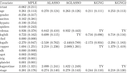
of observed survival times. Table 2.4 gives the estimates of coefficients by five methods: the

maximum partial likelihood estimator (MPLE), the adaptive LASSO (ALASSO) estimator

of Zhang and Lu (2007) based on a standard Cox model, the AGLASSO, and KGNG and

KGNG2 based on a time-varying coefficient Cox model. The numbers given in parenthesis are

the estimated standard errors for important constant coefficients selected by each method. The

results for ALASSO and AGLASSO are copied directly from Yan and Huang (2012). We make

(39)

identifies three covariates with time-varying coefficients and KGNG2 identifies two, in which

edema and logprotime are the common covariates identified by both KGNG and KGNG2. On

the other hand, AGLASSO only selects logbilli as the covariate with time-varying coefficient.

These results partly agree with the findings of Tian et al. (2005), where only 5 covariates:

age, edema, logbili, logalb and logprotime, are considered in their time-varying coefficient Cox

model, and three covariates: edema, logprotime and logbili, are identified as having time-varying

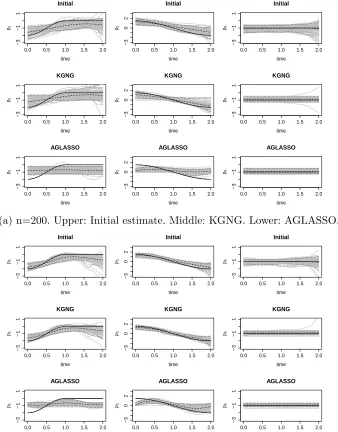
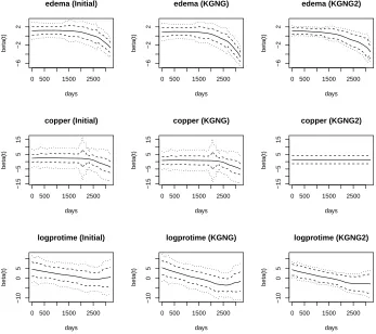
coefficients. Finally, in Figures 2.3 and 2.4, we plotted the estimated coefficients by the initial

step (maximum local partial likelihood estimator), KGNG and KGNG2 for the 7 important

covariates and their associated 95% pointwise confidence intervals and simultaneous confidence

bands.

Table 2.4: Analysis results for PBC data. TV stands for time-varying coefficients.

Covariate MPLE ALASSO AGLASSO KGNG KGNG2

trtmt -0.062 (0.211)

age 0.261 (0.113) 0.270 (0.124) 0.263 (0.126) 0.211 (0.111) 0.253 (0.113) gender -0.256 (0.317)

ascites 0.162 (0.381) hypato -0.100 (0.254) spiders 0.049 (0.243)

edema 0.926 (0.378) 0.842 (0.410) 0.932 (0.443) TV TV

logbili 0.723 (0.162) 0.699 (0.115) TV 0.716 (0.096) 0.718 (0.116) chol 0.000 (0.000)

logalb -2.270 (0.947) -2.538 (0.762) -2.440(0.789) -2.173 (0.934) -2.294 (1.183) copper 1.694 (1.251) 2.218 (1.236) 2.089(1.261) TV 1.379 (1.419)

alk 0.000 (0.000)

sgot 0.003 (0.002) trig -0.002 (0.001) platelet 0.001 (0.001)

logprotime 2.335 (1.321) 2.099 (1.241) 1.822 (1.249) TV TV

(40)

0 500 1500 2500 −6 −2 2 edema (Initial) days beta(t)

0 500 1500 2500

−6 −2 2 edema (KGNG) days beta(t)

0 500 1500 2500

−6 −2 2 edema (KGNG2) days beta(t)

0 500 1500 2500

−15 −5 5 15 copper (Initial) days beta(t)

0 500 1500 2500

−15 −5 5 15 copper (KGNG) days beta(t)

0 500 1500 2500

−15 −5 5 15 copper (KGNG2) days beta(t)

0 500 1500 2500

−10 0 5 logprotime (Initial) days beta(t)

0 500 1500 2500

−10 0 5 logprotime (KGNG) days beta(t)

0 500 1500 2500

−10 0 5 logprotime (KGNG2) days beta(t)

(41)

0 500 1500 2500 −0.5 0.5 age (Initial) days beta(t)

0 500 1500 2500

−0.5

0.5

age (KGNG)

days

beta(t)

0 500 1500 2500

−0.5

0.5

age (KGNG2)

days

beta(t)

0 500 1500 2500

0.0

1.0

logbili (Initial)

days

beta(t)

0 500 1500 2500

0.0

1.0

logbili (KGNG)

days

beta(t)

0 500 1500 2500

0.0

1.0

logbili (KGNG2)

days

beta(t)

0 500 1500 2500

−10 0 5 logalb (Initial) days beta(t)

0 500 1500 2500

−10 0 5 logalb (KGNG) days beta(t)

0 500 1500 2500

−10 0 5 logalb (KGNG2) days beta(t)

0 500 1500 2500

−0.5 0.5 1.5 stage (Initial) days beta(t)

0 500 1500 2500

−0.5 0.5 1.5 stage (KGNG) days beta(t)

0 500 1500 2500

−0.5 0.5 1.5 stage (KGNG2) days beta(t)

(42)

2.5 Discussion

We propose a kernel group nonnegative garrote (KGNG) estimation method and its variant

(KGNG2) for automatic structure selection and coefficient estimation in a time-varying

coef-ficient Cox model. We establish the asymptotic properties, including structure selection

con-sistency and asymptotic distributions, of our estimators for both constant and time-varying

coefficients. Numerical studies have shown the competitive performance of the proposed

meth-ods compared with existing approaches.

In this chapter, we only focus on the case with fixed dimensionp, and pis smaller than the

sample sizen. Forp > ncase, a penalty term needs to be added to (2.2) to get reasonable initial

estimates of the coefficient functions. Then Step 2 and 3 can follow similarly as proposed in this

chapter. For an ultra-high dimension case, say,pn, a screening procedure can be utilized to remove the noisy covariates beforehand. Then the dimension of the model can be decreased to a

value that can be handled directly. However, a screening procedure for time-varying coefficient

Cox model has not yet been developed in the literature, and it needs further investigation.

Since the proposed procedure depends on a large number of tuning parameters, it may be

useful to develop a statistical test to check the goodness-of-fit of the final estimated model. We

think that a cumulative sums of martingale residuals-based goodness-of-fit test can be derived

for the final estimated model, following the techniques of Lin, Wei and Ying (1993). A similar

goodness-of-fit test procedure was developed for the Dantzig selector in Cox’s proportional

hazards model (Antoniadis, Fryzlewicz and Letue, 2010). This is an interesting topic that needs

further investigation.

Another interesting problem, as suggested by a referee, is to extend the proposed methods to

domain selection, i.e., to develop a procedure which estimates the coefficients as exactly zero on

parts of the time domain, and as nonzero (and time-varying) on the remaining parts. One simple

solution would be to chop the coefficient functions evenly into small pieces on the study time

(43)

challenging. The proposed KGNG/KGNG2 methods for structure selection can be regarded

as a preliminary step for domain selection since they can help to remove all the covariates

with null or constant effects and thus achieve effective dimension reduction. Then, the domain

selection can only focus on the selected covariates with truly time-varying coefficients. This is

an interesting extension that warrants our future research.

2.6 Supplement

This supplementary section contains the proofs of Lemma 2.2, and Theorem 2.1, 2.2 and 2.3.

Before we give the details of proofs, we first introduce some additional notation. With simple

matrix multiplication, we have λ(1)₀ =P1λ0 and λ(0)0 =P2λ0, where

P1 = 

    

0p2×p1 Ip2 0p2×p3 0p2×p1 0p2×p2 0p2×p3

0p3×p1 0p3×p2 Ip3 0p3×p1 0p3×p2 0p3×p3

0p3×p1 0p3×p2 0p3×p3 0p3×p1 0p3×p2 Ip3



    

(p2+2p3)×2p

; (2.7)

P2 =



    

Ip1 0p1×p2 0p1×p3 0p1×p1 0p1×p2 0p1×p3

0p1×p1 0p1×p2 0p1×p3 Ip1 0p1×p2 0p1×p3

0p2×p1 0p2×p2 0p2×p3 0p2×p1 Ip2 0p2×p3



    

(2p1+p2)×2p

. (2.8)

Let λ0 = (λ(1)0

T

,λ(0)₀ T)T_{. We also have} _λ

(44)

P41λ(1)+P42λ(0), where

P3 = (P31|P32) =      

0p1×p2 0p1×p3 0p1×p3 Ip1 0p1×p1 0p1×p2

Ip2 0p2×p3 0p2×p3 0p2×p1 0p2×p1 0p2×p2

0p3×p3 Ip3 0p3×p3 0p3×p1 0p3×p1 0p3×p2

     

p×2p

; (2.9)

P4 = (P41|P42) =

     

0p1×p2 0p1×p3 0p1×p3 0p1×p1 Ip1 0p1×p2

0p2×p2 0p2×p3 0p2×p3 0p2×p1 0p2×p1 Ip2

0p3×p2 0p3×p3 Ip3 0p3×p1 0p3×p1 0p3×p2

     

p×2p

. (2.10)

LetL2n(λ1,λ2;fm,βe

∗

(·)) andQ2n(λ1,λ2;fm,βe

∗

(·)) denote the partial likelihood and penal-ized partial likelihood in equation (2.3) respectively. We then have

L2n(λ1,λ2;m,β(·)) =

n X i=1 Z τ 0 

a(s)

T_Z

i−log 

 n X

j=1

Yj(s)ea(s)

T_Z j



 

dNi(s);

Q2n(λ1,λ2;m,β(·)) =−L2n(λ1,λ2;m,β(·)) +θ1kλ1k1+θ2kλ2k1,

where

a(s)≡a(s,λ(1),λ(0);m,β∗(·))≡a(s,λ1,λ2;m,β∗(·)) =λ1◦m+λ2◦β∗(s). (2.11)

Let U(λ1,λ2;m,β∗(·)) and H(λ1,λ2;m,β∗(·)) denote the vector and matrix of the first and

second order partial derivatives of L2n(λ1,λ2;m,β(·)) with respect toλ= (λT1,λT2)T. Thus

U(λ1,λ2;m,β(·)) =

n X i=1 τ Z 0

A(s) (Zi−E(a(s), s))dNi(s),

H(λ1,λ2;m,β(·)) =−

n X i=1 τ Z 0 A(s)





S(2)(a(s), s)

S(0)₍_a₍_s₎_{, s}₎ −

S(1)(a(s), s)

S(0)₍_a₍_s₎_{, s}₎

!⊗2 A(s)

T_dN